Numerical methods challenge: Summary

Nicolás Guarín-Zapata

2017-11-14 11:22

During October (2017) I wrote a program per day for some well-known numerical methods in both Python and Julia. It was intended to be an exercise, then don't expect the code to be good enough for real use. Also, I should mention that I had almost no experience with Julia, so it probably is not idiomatic Julia but more Python-like Julia.

Summary

This post is a summary of that challenge. For the source code you can check the repository.

The verdict

Since the challenge is with myself, and the main purpose was to learn some Julia the verdict is: success. Nevertheless, I failed during day 26 with the Boundary Element Method.

The list of methods

Day	Numerical method
01	Bisection
02	Regula falsi
03	Newton
04	Newton multivariate
05	Broyden
06	Gradient descent
07	Nelder-Mead
08	Newton for optimization
09	Lagrange interpolation
10	Lagrange interpolation with Lobatto sampling
11	Lagrange interpolation using Vandermonde matrix
12	Hermite interpolation
13	Spline interpolation
14	Trapezoid quadrature
15	Simpson quadrature
16	Clenshaw-Curtis quadrature
17	Euler integration
18	Runge-Kutta integration
19	Verlet integration
20	Shooting method
21	Finite differences with Jacobi method
22	Finite differences for eigenvalues
23	Ritz method
24	Finite element method in 1D
25	Finite element method in 2D
26	Boundary element method
27	Monte-Carlo integration
28	LU factorization
29	Cholesky factorization
30	Conjugate gradient
31	Finite element method with solver

Conclusions

This was an exercise of code-kata to learn some of the details of Julia for scientific computing. As such, it was really useful for me to get my hands dirty with Julia.
Implementing the Boundary Element Method in one day seems to be rough. I knew this beforehand, but I gave it a try anyways … without succcess.
Julia syntax is somewhat in a sweetspot between Python and MATLAB. This makes it really easy to use, although the documentation of some packages is at an arcane stage right now.
I won't take a challenge like this in a while. It takes a lot of atttention to get it done.

Numerical methods challenge: Day 31

Nicolás Guarín-Zapata

2017-10-31 20:45

Comments

During October (2017) I wrote a program per day for some well-known numerical methods in both Python and Julia. It was intended to be an exercise, then don't expect the code to be good enough for real use. Also, I should mention that I had almost no experience with Julia, so it probably is not idiomatic Julia but more Python-like Julia.

Putting some things together

Today, I am putting some things together, namely, I am going to solve the system of equations that results in the finite element using the conjugate gradient.

Following are the codes

Python

from __future__ import division, print_function
import numpy as np
import matplotlib.pyplot as plt


def FEM1D(coords, source):
    N = len(coords)
    stiff_loc = np.array([[2.0, -2.0], [-2.0, 2.0]])
    eles = [np.array([cont, cont + 1]) for cont in range(0, N - 1)]
    stiff = np.zeros((N, N))
    rhs = np.zeros(N)
    for ele in eles:
        jaco = coords[ele[1]] - coords[ele[0]]
        rhs[ele] = rhs[ele] + jaco*source(coords[ele])
        for cont1, row in enumerate(ele):
            for cont2, col in enumerate(ele):
                stiff[row, col] = stiff[row, col] +  stiff_loc[cont1, cont2]/jaco
    return stiff, rhs


def conj_grad(A, b, x, tol=1e-8):
    r = b - A.dot(x)
    p = r
    rsq_old = r.dot(r)
    for cont in range(len(b)):
        Ap = A.dot(p)
        alpha = rsq_old / p.dot(Ap)
        x = x + alpha*p
        r = r - alpha*Ap
        rsq_new = r.dot(r)
        if np.sqrt(rsq_new) < tol:
            break
        p = r + (rsq_new / rsq_old) * p
        rsq_old = rsq_new
    return x, cont, np.sqrt(rsq_new)


fun = lambda x: x**3
N_vec = np.logspace(0.5, 3, 50, dtype=int)
err_vec = np.zeros_like(N_vec, dtype=float)
niter_vec = np.zeros_like(N_vec)
plt.figure(figsize=(8, 3))
for cont, N in enumerate(N_vec):
    x = np.linspace(0, 1, N)
    stiff, rhs = FEM1D(x, fun)
    sol = np.zeros(N)
    sol[1:-1], niter, _ = conj_grad(stiff[1:-1, 1:-1], -rhs[1:-1], rhs[1:-1])
    err = np.linalg.norm(sol - x*(x**4 - 1)/20)/np.linalg.norm(x*(x**4 - 1)/20)
    err_vec[cont] = err
    niter_vec[cont] = niter

plt.subplot(121)
plt.loglog(N_vec, err_vec)
plt.xlabel("Number of nodes")
plt.ylabel("Relative error")
plt.subplot(122)
plt.loglog(N_vec, niter_vec)
plt.xlabel("Number of nodes")
plt.ylabel("Number of iterations")
plt.tight_layout()
plt.show()

Julia

using PyPlot


function FEM1D(coords, source)
    N = length(coords)
    stiff_loc = [2.0 -2.0; -2.0 2.0]
    eles = [[cont, cont + 1] for cont in 1:N-1]
    stiff = zeros(N, N)
    rhs = zeros(N)
    for ele in eles
        jaco = coords[ele[2]] - coords[ele[1]]
        rhs[ele] = rhs[ele] + jaco*source(coords[ele])
        stiff[ele, ele] = stiff[ele, ele] +  stiff_loc/jaco
    end
    return stiff, rhs
end


function conj_grad(A, b, x; tol=1e-8)
    r = b - A * x
    p = r
    rsq_old = dot(r, r)
    niter = 1
    for cont = 1:length(b)
        Ap = A * p
        alpha = rsq_old / dot(p, Ap)
        x = x + alpha*p
        r = r - alpha*Ap
        rsq_new = dot(r, r)
        if sqrt(rsq_new) < tol
            break
        end
        p = r + (rsq_new / rsq_old) * p
        rsq_old = rsq_new
        niter += 1
    end
    return x, niter, norm(r)
end



fun(x) = x.^3
N_vec = round.(logspace(0.5, 3, 50))
err_vec = zeros(N_vec)
niter_vec = zeros(N_vec)
figure(figsize=(8, 3))
for (cont, N) in enumerate(N_vec)
    x = linspace(0.0, 1.0,N)
    stiff, rhs = FEM1D(x, fun)
    sol = zeros(N)
    sol[2:end-1], niter, _ = conj_grad(stiff[2:end-1, 2:end-1],
                                -rhs[2:end-1], rhs[2:end-1])
    err = norm(sol - x.*(x.^4 - 1)/20)/norm(x.*(x.^4 - 1)/20)
    err_vec[cont] = err
    niter_vec[cont] = niter
end
subplot(121)
loglog(N_vec, err_vec)
xlabel("Number of nodes")
ylabel("Relative error")
subplot(122)
loglog(N_vec, niter_vec)
xlabel("Number of nodes")
ylabel("Number of iterations")
tight_layout()
show()

In this case, we are analyzing the error of the solution as a function of the number of nodes. This, and the number of iterations required in the conjugate gradient are shown in the following image

Numerical methods challenge: Day 30

Nicolás Guarín-Zapata

2017-10-30 19:38

Comments

During October (2017) I will write a program per day for some well-known numerical methods in both Python and Julia. It is intended to be an exercise then don't expect the code to be good enough for real use. Also, I should mention that I have almost no experience with Julia, so it probably won't be idiomatic Julia but more Python-like Julia.

Conjugate gradient

Today we have the conjugate gradient method. This method is commonly used to solve positive-definite linear systems of equations. Compared with gradient descent, we choose as descent direction a direction that is conjugated with the residual, that is, it is orthogonal with the matrix as weighting.

Following are the codes

Python

from __future__ import division, print_function
import numpy as np


def conj_grad(A, b, x, tol=1e-8):
    r = b - A.dot(x)
    p = r
    rsq_old = r.dot(r)
    for cont in range(len(b)):
        Ap = A.dot(p)
        alpha = rsq_old / p.dot(Ap)
        x = x + alpha*p
        r = r - alpha*Ap
        rsq_new = r.dot(r)
        if np.sqrt(rsq_new) < tol:
            break
        p = r + (rsq_new / rsq_old) * p
        rsq_old = rsq_new
    return x, cont, np.sqrt(rsq_new)


N = 1000
A = -np.diag(2*np.ones(N)) + np.diag(np.ones(N-1), -1) +\
    np.diag(np.ones(N-1), 1)
b = np.ones(N)
x0 = np.ones(N)
x, niter, accu = conj_grad(A, b, x0)

Julia

function conj_grad(A, b, x; tol=1e-8)
    r = b - A * x
    p = r
    rsq_old = dot(r, r)
    niter = 1
    for cont = 1:length(b)
        Ap = A * p
        alpha = rsq_old / dot(p, Ap)
        x = x + alpha*p
        r = r - alpha*Ap
        rsq_new = dot(r, r)
        if sqrt(rsq_new) < tol
            break
        end
        p = r + (rsq_new / rsq_old) * p
        rsq_old = rsq_new
        niter += 1
    end
    return x, niter, norm(r)
end


N = 1000
A = -diagm(2*ones(N)) + diagm(ones(N-1), -1) + diagm(ones(N-1), 1)
b = ones(N)
x0 = ones(N)
x, niter, accu = conj_grad(A, b, x0)

In this case, we are testing the method with a matrix that comes from the discretization of the second order derivative using finite differences.

Comparison Python/Julia

Regarding number of lines we have: 27 in Python and 27 in Julia. The comparison in execution time is done with %timeit magic command in IPython and @benchmark in Julia.

For Python:

%timeit conj_grad(A, b, x0)

with result

10 loops, best of 3: 107 ms per loop

For Julia:

@benchmark conj_grad(A, b, x0)

with result

BenchmarkTools.Trial:
  memory estimate:  27.13 MiB
  allocs estimate:  3501
  --------------
  minimum time:     128.477 ms (0.54% GC)
  median time:      294.407 ms (0.24% GC)
  mean time:        298.208 ms (0.30% GC)
  maximum time:     464.223 ms (0.30% GC)
  --------------
  samples:          17
  evals/sample:     1

In this case, we can say that the Python code is roughly 2 times faster than Julia code.

Numerical methods challenge: Day 29

Nicolás Guarín-Zapata

2017-10-29 21:10

Comments

During October (2017) I will write a program per day for some well-known numerical methods in both Python and Julia. It is intended to be an exercise then don't expect the code to be good enough for real use. Also, I should mention that I have almost no experience with Julia, so it probably won't be idiomatic Julia but more Python-like Julia.

Cholesky decomposition

Today we have Cholesky decomposition. It is a factorization of a Hermitian, positive-definite matrix into a lower and upper matrix, the main difference with LU decomposition is that it the lower matrix is the Hermitian transpose of the upper one.

Following are the codes

Python

from __future__ import division, print_function
import numpy as np


def cholesky(mat):
    m, _ = mat.shape
    mat = mat.copy()
    for col in range(m):
        print(mat[col, col] -
               mat[col, 0:col].dot(mat[col, 0:col]))
        mat[col, col] = np.sqrt(mat[col, col] -
               mat[col, 0:col].dot(mat[col, 0:col]))
        for row in range(col + 1, m):
            mat[row, col] = (mat[row, col] -
               mat[row, 0:col].dot(mat[col, 0:col]))/mat[col, col]
    for row in range(1, m):
        mat[0:row, row] = 0
    return mat


A = np.array([
    [4, -1, 1],
    [-1, 4.25, 2.75],
    [1, 2.75, 3.5]], dtype=float)
B = cholesky(A)

Julia

function cholesky(mat)
    m, _ = size(mat)
    mat = copy(mat)
    for col = 1:m
        mat[col, col] = sqrt(mat[col, col] -
            dot(mat[col, 1:col-1], mat[col, 1:col-1]))
        for row = col + 1:m
            mat[row, col] = (mat[row, col] -
               dot(mat[row, 1:col-1], mat[col, 1:col-1]))/mat[col, col]
        end
    end
    for row = 2:m
        mat[1:row-1, row] = 0
    end
    return mat
end


A = [4 -1 1;
    -1 4.25 2.75;
    1 2.75 3.5]
B = cholesky(A)

As an example we have the matrix

\begin{equation*} A = \begin{bmatrix} 4 &-1 &1\\ -1 &4.25 &2.75\\ 1 &2.75 &3.5 \end{bmatrix} \end{equation*}

And, the answer of both codes is

2.0  0.0  0.0
-0.5  2.0  0.0
0.5  1.5  1.0

Comparison Python/Julia

Regarding number of lines we have: 23 in Python and 22 in Julia. The comparison in execution time is done with %timeit magic command in IPython and @benchmark in Julia.

For Python:

%timeit cholesky(np.eye(100))

with result

100 loops, best of 3: 13 ms per loop

For Julia:

@benchmark cholesky(eye(100))

with result

BenchmarkTools.Trial:
  memory estimate:  4.01 MiB
  allocs estimate:  20303
  --------------
  minimum time:     1.010 ms (0.00% GC)
  median time:      1.136 ms (0.00% GC)
  mean time:        1.370 ms (17.85% GC)
  maximum time:     4.652 ms (40.37% GC)
  --------------
  samples:          3637
  evals/sample:     1

In this case, we can say that the Python code is roughly 10 times slower than Julia code.

Numerical methods challenge: Day 28

Nicolás Guarín-Zapata

2017-10-28 17:02

Comments

During October (2017) I will write a program per day for some well-known numerical methods in both Python and Julia. It is intended to be an exercise then don't expect the code to be good enough for real use. Also, I should mention that I have almost no experience with Julia, so it probably won't be idiomatic Julia but more Python-like Julia.

LU factorization

Today we have LU decomposition. That is a factorization of a matrix into a lower (L) and upper (U) matrix. Basically it stores de steps of a Gauss elimination in matrices.

Following are the codes

Python

from __future__ import division, print_function
import numpy as np


def LU(mat):
    m, _ = mat.shape
    mat = mat.copy()
    for col in range(0, m - 1):
        for row in range(col + 1, m):
            if mat[row, col] != 0.0:
                lam = mat[row, col]/mat[col, col]
                mat[row, col + 1:m] = mat[row, col + 1:m] -\
                                      lam * mat[col, col + 1:m]
                mat[row, col] = lam
    return mat


A = np.array([
    [1, 1, 0, 3],
    [2, 1, -1, 1],
    [3, -1, -1, 2],
    [-1, 2, 3, -1]], dtype=float)
B = LU(A)

Julia

function LU(mat)
    m, _ = size(mat)
    mat = copy(mat)
    for col = 1:m - 2
        for row = col + 1:m
            if mat[row, col] != 0.0
                lam = mat[row, col]/mat[col, col]
                mat[row, col + 1:m] = mat[row, col + 1:m] -
                                      lam * mat[col, col + 1:m]
                mat[row, col] = lam
            end
        end
    end
    return mat
end


A = [1.0 1.0 0.0 3.0;
    2.0 1.0 -1.0 1.0;
    3.0 -1.0 -1.0 2.0;
    -1.0 2.0 3.0 -1.0]
B = LU(A)

As an example we have the matrix

\begin{equation*} A = \begin{bmatrix} 1 &1 &0 &3\\ 2 &1 &-1 &1\\ 3 &-1 &-1 &2\\ -1 &2 &3 &-1 \end{bmatrix} = \begin{bmatrix} 1 &1 &0 &0\\ 2 &1 &0 &0\\ 3 &4 &1 &2\\ -1 &-3 &0 &1 \end{bmatrix} \begin{bmatrix} 1 &1 &0 &3\\ 0 &-1 &-1 &-5\\ 0 &0 &3 &13\\ 0 &0 &0 &-13 \end{bmatrix} \end{equation*}

And, the answer of both codes is

[[  1.,   1.,   0.,   3.],
 [  2.,  -1.,  -1.,  -5.],
 [  3.,   4.,   3.,  13.],
 [ -1.,  -3.,   0., -13.]]

Comparison Python/Julia

Regarding number of lines we have: 23 in Python and 22 in Julia. The comparison in execution time is done with %timeit magic command in IPython and @benchmark in Julia.

For Python:

%timeit LU(np.random.rand(10, 10))

with result

1000 loops, best of 3: 303 µs per loop

For Julia:

@benchmark LU(rand(10, 10))

with result

BenchmarkTools.Trial:
  memory estimate:  29.25 KiB
  allocs estimate:  310
  --------------
  minimum time:     9.993 μs (0.00% GC)
  median time:      11.725 μs (0.00% GC)
  mean time:        14.943 μs (15.90% GC)
  maximum time:     3.285 ms (95.64% GC)
  --------------
  samples:          10000
  evals/sample:     1

In this case, we can say that the Python code is roughly 30 times slower than Julia code.

Numerical methods challenge: Day 27

Nicolás Guarín-Zapata

2017-10-27 21:27

Comments

During October (2017) I will write a program per day for some well-known numerical methods in both Python and Julia. It is intended to be an exercise then don't expect the code to be good enough for real use. Also, I should mention that I have almost no experience with Julia, so it probably won't be idiomatic Julia but more Python-like Julia.

Monte Carlo integration

Today we have Monte Carlo integration. Where we use random sampling to numerically compute an integral. This method is important when we want to evaluate higher-dimensional integrals since common quadrature techniques imply an exponential growing in the number of sampling points.

The method computes an integral

\begin{equation*} I = \int_\Omega f(x) dx \end{equation*}

where \(\Omega\) has volume \(V\).

The integral is approximated as

\begin{equation*} I \approx \frac{V}{N} \sum_{i=1}^{N} f(x_i) \end{equation*}

where the \(x_i\) distribute uniform over \(\Omega\).

Following are the codes

Python

from __future__ import division, print_function
import numpy as np


def monte_carlo_int(fun, N, low, high, args=()):
    ndims = len(low)
    pts = np.random.uniform(low=low, high=high, size=(N, ndims))
    V = np.prod(np.asarray(high) - np.asarray(low))
    return V*np.sum(fun(pts, *args))/N


def circ(x, rad):
    return 0.5*(1 - np.sign(x[:, 0]**2 + x[:, 1]**2 - rad**2))


N = 1000000
low = [-1, -1]
high = [1, 1]
rad = 1
inte = monte_carlo_int(circ, N, low, high, args=(rad,))

Julia

using Distributions


function monte_carlo_int(fun, N, low, high; args=())
    ndims = length(low)
    pts = rand(Uniform(0, 1), N, ndims)
    for cont = 1:ndims
        pts[:, cont] = pts[:, cont]*(high[cont] - low[cont]) + low[cont]
    end
    V = prod(high - low)
    return V*sum(fun(pts, args...))/N
end


function circ(x, rad)
    return 0.5*(1 - sign.(x[:, 1].^2 + x[:, 2].^2 - rad^2))
end


N = 1000000
low = [-1, -1]
high = [1, 1]
rad = 1
inte = monte_carlo_int(circ, N, low, high, args=(rad,))

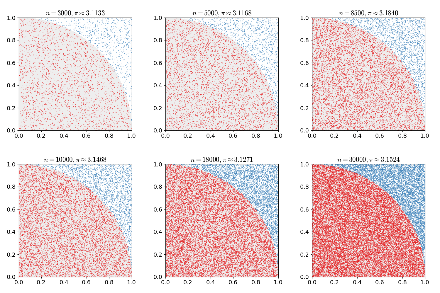
One of the most common examples is the computation of \(\pi\), this is illustrated in the following animation.

Comparison Python/Julia

Regarding number of lines we have: 20 in Python and 24 in Julia. The comparison in execution time is done with %timeit magic command in IPython and @benchmark in Julia.

For Python:

%timeit monte_carlo_int(circ, N, low, high, args=(rad,))

with result

10 loops, best of 3: 53.2 ms per loop

For Julia:

@benchmark monte_carlo_int(circ, N, low, high, args=(rad,))

with result

BenchmarkTools.Trial:
  memory estimate:  129.70 MiB
  allocs estimate:  46
  --------------
  minimum time:     60.131 ms (5.15% GC)
  median time:      164.018 ms (55.64% GC)
  mean time:        204.366 ms (49.50% GC)
  maximum time:     357.749 ms (64.04% GC)
  --------------
  samples:          25
  evals/sample:     1

In this case, we can say that the Python code is roughly 3 times faster than Julia code.

Numerical methods challenge: Day 26

Nicolás Guarín-Zapata

2017-10-26 19:15

Comments

During October (2017) I will write a program per day for some well-known numerical methods in both Python and Julia. It is intended to be an exercise then don't expect the code to be good enough for real use. Also, I should mention that I have almost no experience with Julia, so it probably won't be idiomatic Julia but more Python-like Julia.

Boundary element method

Today we have the Boundary element method , or, an attempt. We want so solve the equation

\begin{equation*} \nabla^2 u = -f(x) \end{equation*}

with

\begin{equation*} u(x) = g(x),\quad \forall (x, y)\in \partial \Omega \end{equation*}

For this method, we need to use an integral representation of the equation, that in this case is

\begin{equation*} u(\xi) = \int_{S} [u(x) F(x, \xi) - q(x)G(x, \xi)]dS(x) + \int_{V} f(x) G(x, \xi) dV(x) \end{equation*}

with

\begin{equation*} G(x,\xi)= -\frac{1}{2\pi}\ln|x- \xi| \end{equation*}

and

\begin{equation*} F(x,\xi) = -\frac{1}{2\pi |x- \xi|^2}(x - \xi)\cdot\hat{n} \end{equation*}

Then, we can form a system of equations

\begin{equation*} [G]\{q\} = [F]\{u\}\, , \end{equation*}

that we obtain by discretization of the boundary. If we take constant variables over the discretization, the integral can be computed analytically by

\begin{equation*} G_{nm} = -\frac{1}{2\pi}\left[r \sin\theta\left(\ln|r| - 1\right) + \theta r\cos\theta\right]^{\theta_B, r_B}_{\theta_A, r_A} \end{equation*}

and

\begin{equation*} F_{nm} = \left[\frac{\theta}{2\pi}\right]^{\theta_B}_{\theta_A} \end{equation*}

for points \(n\) and \(m\) in different elements, and the subindices \(A,B\) refer to the endpoints of the evaluation element. For diagonal terms the integrals evaluate to

\begin{equation*} G_{nn} = -\frac{L}{2\pi}\left(\ln\left\vert\frac{L}{2}\right\vert - 1\right) \end{equation*}

and

\begin{equation*} F_{nn} = - \frac{1}{2\pi} \end{equation*}

with \(L\) the size of the element.

Below is the Python code. In this case, I did not succeed and the code is not working right now.

from __future__ import division, print_function
import numpy as np
from numpy import log, sin, cos, arctan2, pi, mean, arctan
from numpy.linalg import norm, solve
import matplotlib.pyplot as plt


def assem(coords, elems):
    nelems = elems.shape[0]
    Gmat = np.zeros((nelems, nelems))
    Fmat = np.zeros((nelems, nelems))
    for ev_cont, elem1 in enumerate(elems):
        print(coords[elem1[0]], coords[elem1[1]])
        for col_cont, elem2 in enumerate(elems):
            pt_col = mean(coords[elem2], axis=0)
            if ev_cont == col_cont:
                L = norm(coords[elem1[1]] - coords[elem1[0]])
                Gmat[ev_cont, ev_cont] = - L/(2*pi)*(log(L/2) - 1)
                Fmat[ev_cont, ev_cont] = - 0.5
            else:
                Gij, Fij = influence_coeff(elem1, coords, pt_col)
                Gmat[ev_cont, col_cont] = Gij
                Fmat[ev_cont, col_cont] = Fij
    return Gmat, Fmat


def influence_coeff(elem, coords, pt_col):
    r_A = coords[elem[0]] - pt_col
    r_B = coords[elem[1]] - pt_col
    theta_A = arctan2(r_A[1], r_A[0])
    theta_B = arctan2(r_B[1], r_B[0])
    G_coeff = r_B[1]*(log(norm(r_B)) - 1) + theta_B*r_B[0] -\
              (r_A[1]*(log(norm(r_A)) - 1) + theta_A*r_A[0])
    F_coeff = theta_B - theta_A
    return -G_coeff/(2*pi), F_coeff/(2*pi)


def eval_sol(ev_coords, coords):
    nelems = elems.shape[0]
    Gmat = np.zeros((nelems, nelems))
    Fmat = np.zeros((nelems, nelems))
    for ev_cont, elem1 in enumerate(elems):
        L = norm(coords[elem1[1]] - coords[elem1[0]])
        for col_cont, elem2 in enumerate(elems):
            pt_col = mean(coords[elem2], axis=0)
            if ev_cont == col_cont:
                Gmat[ev_cont, ev_cont] = - L/(2*pi)*(log(L/2) - 1)
                Fmat[ev_cont, ev_cont] = - 0.5
            else:
                Gmat[ev_cont, col_cont], Fmat[ev_cont, col_cont] = \
                    influence_coeff(elem1, coords, pt_col)

nelems = 3
rad = 1.0
theta =  np.linspace(0, 2*pi, nelems, endpoint=False)
coords = rad * np.vstack((cos(theta), sin(theta))).T
elems = np.array([[cont, (cont + 1)%nelems] for cont in range(nelems)])
Gmat, Fmat = assem(coords, elems)
u_boundary = np.ones_like(theta)
q_boundary = solve(Gmat, Fmat.dot(u_boundary))

Numerical methods challenge: Day 25

Nicolás Guarín-Zapata

2017-10-25 21:41

Comments

During October (2017) I will write a program per day for some well-known numerical methods in both Python and Julia. It is intended to be an exercise then don't expect the code to be good enough for real use. Also, I should mention that I have almost no experience with Julia, so it probably won't be idiomatic Julia but more Python-like Julia.

Finite element method

Today we have the Finite element method to solve the equation:

\begin{equation*} \nabla^2 u = -f(x) \end{equation*}

with

\begin{equation*} u(\sqrt{3}, 1) = 0 \end{equation*}

As in the Ritz method we form a functional that is equivalent to the differential equation, propose an approximation as a linear combination of a set of basis functions and find the best set of coefficients for that combination. That best solution is found minimizing the functional.

The functional for this differential equation is

\begin{equation*} \Pi[u] = -\int_\Omega \left(\nabla u\right)^2 d\Omega -\int_\Omega u f(x) d\Omega \end{equation*}

Using linear triangles, the local stiffness matrices read

\begin{equation*} K_\text{local} = \frac{1}{2|J|} \begin{bmatrix} 2 & -1 &1\\ -1 & 1 &0\\ -1 & 0 &1\\ \end{bmatrix} \end{equation*}

and

\begin{equation*} b_\text{local} = -|J| f(x_m) \mathbf{1}_3\, , \end{equation*}

where \(|J|\) is the Jacobian determinant of the transformation and \(x_m\) is the centroid of the triangle. I am skipping a great deal about assembling, but it would be just too extensive to describe the complete process.

We will solve the problem in a mesh with 6 triangles forming a regular hexagon

Following are the codes.

Python

from __future__ import division, print_function
import numpy as np
import matplotlib.pyplot as plt

def assem(coords, elems, source):
    ncoords = coords.shape[0]
    stiff = np.zeros((ncoords, ncoords))
    rhs = np.zeros((ncoords))
    for el_cont, elem in enumerate(elems):
        stiff_loc, jaco = local_stiff(coords[elem])
        rhs[elem] += jaco*np.mean(source[elem])
        for row in range(3):
            for col in range(3):
                row_glob, col_glob = elem[row], elem[col]
                stiff[row_glob, col_glob] += stiff_loc[row, col]
    return stiff, rhs


def local_stiff(coords):
    dHdr = np.array([[-1, 1, 0], [-1, 0, 1]])
    jaco = dHdr.dot(coords)
    stiff = 0.5*np.array([[2, -1, -1], [-1, 1, 0], [-1, 0, 1]])
    return stiff/np.linalg.det(jaco), np.linalg.det(jaco)


sq3 = np.sqrt(3)
coords = np.array([
        [sq3, -1],
        [0, 0],
        [2*sq3, 0],
        [0, 2],
        [2*sq3, 2],
        [sq3, 3],
        [sq3, 1]])
elems = np.array([
        [1, 0, 6],
        [0, 2, 6],
        [2, 4, 6],
        [4, 5, 6],
        [5, 3, 6],
        [3, 1, 6]])
source = -np.ones(7)
stiff, rhs = assem(coords, elems, source)
free = range(6)
sol = np.linalg.solve(stiff[np.ix_(free, free)], rhs[free])
sol_c = np.zeros(coords.shape[0])
sol_c[free] = sol
plt.tricontourf(coords[:, 0], coords[:, 1], sol_c, cmap="hot")
plt.colorbar()
plt.axis("image")
plt.show()

Julia

using PyPlot


function assem(coords, elems, source)
    ncoords = size(coords)[1]
    nelems = size(elems)[1]
    stiff = zeros(ncoords, ncoords)
    rhs = zeros(ncoords)
    for el_cont = 1:nelems
        elem = elems[el_cont, :]
        stiff_loc, jaco = local_stiff(coords[elem, :])
        rhs[elem] += jaco*mean(source[elem])
        for row = 1:3
            for col = 1:3
                row_glob = elem[row]
                col_glob = elem[col]
                stiff[row_glob, col_glob] += stiff_loc[row, col]
            end
        end
    end
    return stiff, rhs
end


function local_stiff(coords)
    dHdr = [-1 1 0; -1 0 1]
    jaco = dHdr * coords
    stiff = 0.5*[2 -1 -1; -1 1 0; -1 0 1]
    return stiff/det(jaco), det(jaco)
end


sq3 = sqrt(3)
coords =[sq3 -1;
        0 0;
        2*sq3 0;
        0 2;
        2*sq3 2;
        sq3 3;
        sq3 1]
elems =[2 1 7;
        1 3 7;
        3 5 7;
        5 6 7;
        6 4 7;
        4 2 7]
source = -ones(7)
stiff, rhs = assem(coords, elems, source)
free = 1:6
sol = stiff[free, free] \ rhs[free]
sol_c = zeros(size(coords)[1])
sol_c[free] = sol
tricontourf(coords[:, 1], coords[:, 2], sol_c, cmap="hot")
colorbar()
axis("image")
show()

Both have the same result, as follows

Comparison Python/Julia

Regarding number of lines we have: 51 in Python and 56 in Julia. The comparison in execution time is done with %timeit magic command in IPython and @benchmark in Julia. For the test we are just comparing the time it takes to generate the matrices.

For Python:

%timeit assem(coords, elems, source)

with result

1000 loops, best of 3: 671 µs per loop

For Julia:

@benchmark assem(coords, elems, source)

with result

BenchmarkTools.Trial:
  memory estimate:  13.30 KiB
  allocs estimate:  179
  --------------
  minimum time:     7.777 μs (0.00% GC)
  median time:      8.934 μs (0.00% GC)
  mean time:        10.810 μs (14.54% GC)
  maximum time:     797.432 μs (95.85% GC)
  --------------
  samples:          10000
  evals/sample:     4

In this case, we can say that the Python code is about 70 times slower than Julia code.

Numerical methods challenge: Day 24

Nicolás Guarín-Zapata

2017-10-24 15:17

Comments

During October (2017) I will write a program per day for some well-known numerical methods in both Python and Julia. It is intended to be an exercise then don't expect the code to be good enough for real use. Also, I should mention that I have almost no experience with Julia, so it probably won't be idiomatic Julia but more Python-like Julia.

Finite element method

Today we have the Finite element method to solve the equation:

\begin{equation*} \frac{d^2 u}{dx^2} = f(x) \end{equation*}

with

\begin{equation*} u(0) = u(1) = 0 \end{equation*}

As in the Ritz method we form a functional that is equivalent to the differential equation, propose an approximation as a linear combination of a set of basis functions and find the best set of coefficients for that combination. That best solution is found minimizing the functional.

The functional for this differential equation is

\begin{equation*} \Pi[u] = -\int_{0}^{1} \left(\frac{d u}{d x}\right)^2 dx -\int_{0}^{1} u f(x) dx \end{equation*}

The main difference is that we use a piecewise interpolation for the basis functions,

\begin{equation*} \hat{u}(x) = \sum_{n=0}^{N} u_n N_n(x)\, , \end{equation*}

this leads to the system of equations

\begin{equation*} [K]\{\mathbf{c}\} = \{\mathbf{b}\} \end{equation*}

where the local stiffness matrices read

\begin{equation*} K_\text{local} = \frac{1}{|J|}\begin{bmatrix} 2 & -2\\ -2 &2\end{bmatrix} \end{equation*}

and

\begin{equation*} b_\text{local} = -|J|\begin{bmatrix} f(x_m)\\ f(x_{n})\end{bmatrix}\, , \end{equation*}

where \(|J|\) is the Jacobian determinant of the transformation. I am skipping a great deal about assembling, but it would be just too extensive to describe the complete process.

We will test the implementation with the function \(f(x) = x^3\), that leads to the solution

\begin{equation*} u(x) = \frac{x (x^4 - 1)}{20} \end{equation*}

Following are the codes.

Python

from __future__ import division, print_function
import numpy as np
import matplotlib.pyplot as plt


def FEM1D(coords, source):
    N = len(coords)
    stiff_loc = np.array([[2.0, -2.0], [-2.0, 2.0]])
    eles = [np.array([cont, cont + 1]) for cont in range(0, N - 1)]
    stiff = np.zeros((N, N))
    rhs = np.zeros(N)
    for ele in eles:
        jaco = coords[ele[1]] - coords[ele[0]]
        rhs[ele] = rhs[ele] + jaco*source(coords[ele])
        for cont1, row in enumerate(ele):
            for cont2, col in enumerate(ele):
                stiff[row, col] = stiff[row, col] +  stiff_loc[cont1, cont2]/jaco
    return stiff, rhs


N = 100
fun = lambda x: x**3
x = np.linspace(0, 1, N)
stiff, rhs = FEM1D(x, fun)
sol = np.zeros(N)
sol[1:-1] = np.linalg.solve(stiff[1:-1, 1:-1], -rhs[1:-1])


#%% Plotting
plt.figure(figsize=(4, 3))
plt.plot(x, sol)
plt.plot(x, x*(x**4 - 1)/20, linestyle="dashed")
plt.xlabel(r"$x$")
plt.ylabel(r"$y$")
plt.legend(["FEM solution", "Exact solution"])
plt.tight_layout()
plt.show()

Julia

using PyPlot


function FEM1D(coords, source)
    N = length(coords)
    stiff_loc = [2.0 -2.0; -2.0 2.0]
    eles = [[cont, cont + 1] for cont in 1:N-1]
    stiff = zeros(N, N)
    rhs = zeros(N)
    for ele in eles
        jaco = coords[ele[2]] - coords[ele[1]]
        rhs[ele] = rhs[ele] + jaco*source(coords[ele])
        stiff[ele, ele] = stiff[ele, ele] +  stiff_loc/jaco
    end
    return stiff, rhs
end


N = 100
fun(x) = x.^3
x = linspace(0, 1, N)
stiff, rhs = FEM1D(x, fun)
sol = zeros(N)
sol[2:end-1] = -stiff[2:end-1, 2:end-1]\rhs[2:end-1]


#%% Plotting
figure(figsize=(4, 3))
plot(x, sol)
plot(x, x.*(x.^4 - 1)/20, linestyle="dashed")
xlabel(L"$x$")
ylabel(L"$y$")
legend(["FEM solution", "Exact solution"])
tight_layout()
show()

Both have the same result, as follows

Comparison Python/Julia

Regarding number of lines we have: 37 in Python and 35 in Julia. The comparison in execution time is done with %timeit magic command in IPython and @benchmark in Julia. For the test we are just comparing the time it takes to generate the matrices.

For Python:

%timeit FEM1D(x, fun)

with result

100 loops, best of 3: 2.15 ms per loop

For Julia:

@benchmark FEM1D(x, fun)

with result

BenchmarkTools.Trial:
  memory estimate:  183.73 KiB
  allocs estimate:  1392
  --------------
  minimum time:     60.045 μs (0.00% GC)
  median time:      70.445 μs (0.00% GC)
  mean time:        98.276 μs (25.64% GC)
  maximum time:     4.269 ms (96.70% GC)
  --------------
  samples:          10000
  evals/sample:     1

In this case, we can say that the Python code is roughly 30 times slower than Julia code.

Numerical methods challenge: Day 23

Nicolás Guarín-Zapata

2017-10-23 20:30

Comments

During October (2017) I will write a program per day for some well-known numerical methods in both Python and Julia. It is intended to be an exercise then don't expect the code to be good enough for real use. Also, I should mention that I have almost no experience with Julia, so it probably won't be idiomatic Julia but more Python-like Julia.

Ritz method

Today we have the Ritz method to solve the equation:

\begin{equation*} \frac{d^2 u}{dx^2} = f(x) \end{equation*}

with

\begin{equation*} u(0) = u(1) = 0 \end{equation*}

The method consist in forming a functional that is equivalent to the differential equation, propose an approximation as a linear combination of a set of basis functions and find the best set of coefficients for that combination. That best solution is found minimizing the functional.

The functional for this differential equation is

\begin{equation*} \Pi[u] = -\int_{0}^{1} \left(\frac{d u}{d x}\right)^2 dx -\int_{0}^{1} u f(x) dx \end{equation*}

In this case, we are using the approximation

\begin{equation*} \hat{u}(x) = x (1 - x)\sum_{n=0}^{N} c_n x^n\, , \end{equation*}

where we picked the factor \(x (1 - x)\) to enforce that the basis functions satisfy the boundary conditions. The approximated functional reads

\begin{align*} \Pi[\hat{u}] = -\sum_{n=0}^{N} \sum_{m=0}^{N} c_n c_m \left[\frac{2 + 2m + 2n + 2mn}{(n + m + 1)(n + m + 2)(n + m +3)}\right] -\\ \sum_{n=0}^{N} c_n\int_{0}^{1} x^{n + 1}(1 - x) f(x) dx \end{align*}

where, in general, we will need to perform numerical integration for the second term.

Minimizing the functional

\begin{equation*} \frac{\partial \Pi[\hat{u}]}{\partial c_m} = 0\, , \end{equation*}

we obtain the system of equations

\begin{equation*} [K]\{\mathbf{c}\} = \{\mathbf{b}\} \end{equation*}

with

\begin{equation*} K_{mn} = \frac{2 + 2m + 2n + 2mn}{(n + m + 1)(n + m + 2)(n + m +3)} \end{equation*}

and

\begin{equation*} b_m = -\int_{0}^{1} x^{m + 1}(1 - x) f(x) dx\, . \end{equation*}

We will test the implementation with the function \(f(x) = x^3\), that leads to the solution

\begin{equation*} u(x) = \frac{x (x^4 - 1)}{20} \end{equation*}

Following are the codes.

Python

from __future__ import division, print_function
import numpy as np
from scipy.integrate import quad
from scipy.linalg import solve
import matplotlib.pyplot as plt


def ritz(N, source):
    stiff_mat = np.zeros((N, N))
    rhs = np.zeros((N))
    for row in range(N):
        for col in range(N):
            numer = (2 + 2*row + 2*col + 2*row*col)
            denom = (row + col + 1) * (row + col + 2) * (row + col + 3)
            stiff_mat[row, col] = numer/denom
        fun = lambda x: x**(row + 1)*(1 - x)*source(x)
        rhs[row], _ = quad(fun, 0, 1)
    return stiff_mat, rhs


N = 2
source = lambda x: x**3
mat, rhs = ritz(N, source)
c = solve(mat, -rhs)
x = np.linspace(0, 1, 100)
y = np.zeros_like(x)
for cont in range(N):
    y += c[cont]*x**(cont + 1)*(1 - x)

#%% Plotting
plt.figure(figsize=(4, 3))
plt.plot(x, y)
plt.plot(x, x*(x**4 - 1)/20, linestyle="dashed")
plt.xlabel(r"$x$")
plt.ylabel(r"$y$")
plt.legend(["Ritz solution", "Exact solution"])
plt.tight_layout()
plt.show()

Julia

using PyPlot


function ritz(N, source)
    stiff_mat = zeros(N, N)
    rhs = zeros(N)
    for row in 0:N-1
        for col in 0:N-1
            numer = (2 + 2*row + 2*col + 2*row*col)
            denom = (row + col + 1) * (row + col + 2) * (row + col + 3)
            stiff_mat[row + 1, col + 1] = numer/denom
        end
        fun(x) = x^(row + 1)*(1 - x)*source(x)
        rhs[row + 1], _  = quadgk(fun, 0, 1)
    end
    return stiff_mat, rhs
end


N = 2
source(x) = x^3
mat, rhs = ritz(N, source)
c = -mat\rhs
x = linspace(0, 1, 100)
y = zeros(x)
for cont in 0:N - 1
    y += c[cont + 1]*x.^(cont + 1).*(1 - x)
end

#%% Plotting
figure(figsize=(4, 3))
plot(x, y)
plot(x, x.*(x.^4 - 1)/20, linestyle="dashed")
xlabel(L"$x$")
ylabel(L"$y$")
legend(["Ritz solution", "Exact solution"])
tight_layout()
show()

Both have (almost) the same result, as follows

Ritz method approximation using 2 terms.

And if we consider 3 terms in the expansion, we get

Ritz method approximation using 3 terms.

Comparison Python/Julia

Regarding number of lines we have: 38 in Python and 38 in Julia. The comparison in execution time is done with %timeit magic command in IPython and @benchmark in Julia.

For Python:

%%timeit
mat, rhs = ritz(5, source)
c = solve(mat, -rhs)

with result

1000 loops, best of 3: 228 µs per loop

For Julia:

function bench()
   mat, rhs = ritz(N, source)
   c = -mat\rhs
end
@benchmark bench()

with result

BenchmarkTools.Trial:
  memory estimate:  6.56 KiB
  allocs estimate:  340
  --------------
  minimum time:     13.527 μs (0.00% GC)
  median time:      15.927 μs (0.00% GC)
  mean time:        17.133 μs (4.50% GC)
  maximum time:     2.807 ms (97.36% GC)
  --------------
  samples:          10000
  evals/sample:     1

In this case, we can say that the Python code is roughly 14 times slower than Julia.