Numerical methods challenge: Day 27 - Monte Carlo integration
During October (2017) I will write a program per day for some well-known numerical methods in both Python and Julia. It is intended to be an exercise then don't expect the code to be good enough for real use. Also, I should mention that I have almost no experience with Julia, so it probably won't be idiomatic Julia but more Python-like Julia.
Monte Carlo integration
Today we have Monte Carlo integration. Where we use random sampling to numerically compute an integral. This method is important when we want to evaluate higher-dimensional integrals since common quadrature techniques imply an exponential growing in the number of sampling points.
The method computes an integral
where \(\Omega\) has volume \(V\).
The integral is approximated as
where the \(x_i\) distribute uniform over \(\Omega\).
Following are the codes
Python
from __future__ import division, print_function
import numpy as np


def monte_carlo_int(fun, N, low, high, args=()):
    ndims = len(low)
    pts = np.random.uniform(low=low, high=high, size=(N, ndims))
    V = np.prod(np.asarray(high) - np.asarray(low))
    return V*np.sum(fun(pts, *args))/N


def circ(x, rad):
    return 0.5*(1 - np.sign(x[:, 0]**2 + x[:, 1]**2 - rad**2))


N = 1000000
low = [-1, -1]
high = [1, 1]
rad = 1
inte = monte_carlo_int(circ, N, low, high, args=(rad,))
Julia
using Distributions


function monte_carlo_int(fun, N, low, high; args=())
    ndims = length(low)
    pts = rand(Uniform(0, 1), N, ndims)
    for cont = 1:ndims
        pts[:, cont] = pts[:, cont]*(high[cont] - low[cont]) + low[cont]
    end
    V = prod(high - low)
    return V*sum(fun(pts, args...))/N
end


function circ(x, rad)
    return 0.5*(1 - sign.(x[:, 1].^2 + x[:, 2].^2 - rad^2))
end


N = 1000000
low = [-1, -1]
high = [1, 1]
rad = 1
inte = monte_carlo_int(circ, N, low, high, args=(rad,))
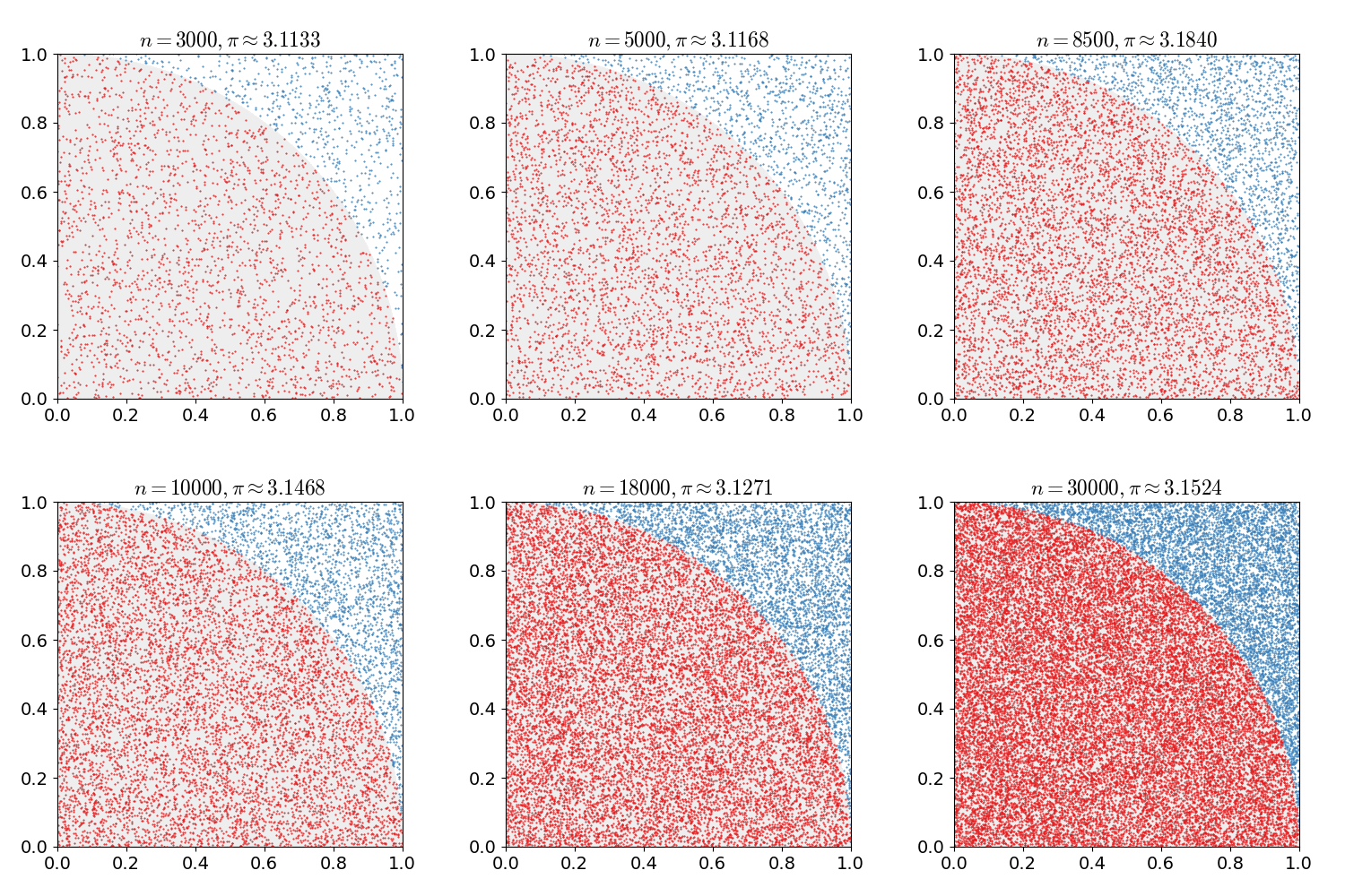
One of the most common examples is the computation of \(\pi\), this is illustrated in the following animation.

Comparison Python/Julia
Regarding number of lines we have: 20 in Python and 24 in Julia. The comparison
in execution time is done with %timeit magic command in IPython and
@benchmark in Julia.
For Python:
with result
For Julia:
with result
BenchmarkTools.Trial:
  memory estimate:  129.70 MiB
  allocs estimate:  46
  --------------
  minimum time:     60.131 ms (5.15% GC)
  median time:      164.018 ms (55.64% GC)
  mean time:        204.366 ms (49.50% GC)
  maximum time:     357.749 ms (64.04% GC)
  --------------
  samples:          25
  evals/sample:     1
In this case, we can say that the Python code is roughly 3 times faster than Julia code.
Comments
Comments powered by Disqus