Coming back to the Boundary element method
During October (2017) I wrote a program per day for some well-known numerical methods in both Python and Julia. It was intended to be an exercise to learn some Julia. You can see a summary here. I succeeded in 30 of the challenges, except for the BEM (Boundary Element Method), where I could not figure out what was wrong that day. The original post is here.
Thomas Klimpel found the mistake and wrote an email where he described my mistakes. So, I am creating a new post with a correct implementation of the BEM.
The Boundary Element Method
We want so solve the equation
with
For this method, we need to use an integral representation of the equation, that, in this case, is
with
and
Then, we can form a system of equations
that we obtain by discretization of the boundary. If we take constant variables over the discretization, the integral can be computed analytically by
and
for points \(n\) and \(m\) in different elements, and the subindices \(A,B\) refer to the endpoints of the evaluation element. We should be careful evaluating this expression since both \(r_A\) and \(r_B\) can be (close to) zero and make it explode. Also, here it was the main problem since I forgot to compute the angles with respect to elements that are, in general, not aligned with horizontal or vertical axes.
For diagonal terms the integrals evaluate to
and
with \(L\) the size of the element.
Following is the code. Keep in mind that this code works for purely Dirichlet problems. For mixed Dirichlet-Neumann the influence matrices would need rearranging to separate known and unknowns in opposite sides of the equation.
You can download the files for this project here. It includes a YML file to create a conda environment with the dependencies listed. For example, it uses version 3.0 of Meshio.
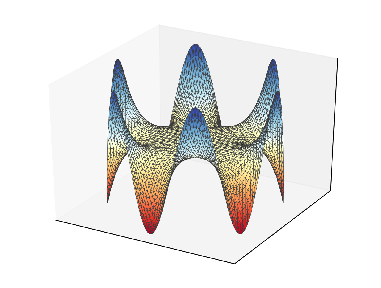
import numpy as np
from numpy import log, arctan2, pi, mean, arctan
from numpy.linalg import norm, solve
import matplotlib.pyplot as plt
from mpl_toolkits.mplot3d import Axes3D
import meshio


  def assem(coords, elems):
      """Assembly matrices for the BEM problem

      Parameters
      ----------
      coords : ndarray, float
          Coordinates for the nodes.
      elems : ndarray, int
          Connectivity for the elements.

      Returns
      -------
      Gmat : ndarray, float
          Influence matrix for the flow.
      Fmat : ndarray, float
          Influence matrix for primary variable.
      """
      nelems = elems.shape[0]
      Gmat = np.zeros((nelems, nelems))
      Fmat = np.zeros((nelems, nelems))
      for ev_cont, elem1 in enumerate(elems):
          for col_cont, elem2 in enumerate(elems):
              pt_col = mean(coords[elem2], axis=0)
              if ev_cont == col_cont:
                  L = norm(coords[elem1[1]] - coords[elem1[0]])
                  Gmat[ev_cont, ev_cont] = - L/(2*pi)*(log(L/2) - 1)
                  Fmat[ev_cont, ev_cont] = - 0.5
              else:
                  Gij, Fij = influence_coeff(elem1, coords, pt_col)
                  Gmat[ev_cont, col_cont] = Gij
                  Fmat[ev_cont, col_cont] = Fij
      return Gmat, Fmat


  def influence_coeff(elem, coords, pt_col):
      """Compute influence coefficients

      Parameters
      ----------
      elems : ndarray, int
          Connectivity for the elements.
      coords : ndarray, float
          Coordinates for the nodes.
      pt_col : ndarray
          Coordinates of the colocation point.

      Returns
      -------
      G_coeff : float
          Influence coefficient for flows.
      F_coeff : float
          Influence coefficient for primary variable.
      """
      dcos = coords[elem[1]] - coords[elem[0]]
      dcos = dcos / norm(dcos)
      rotmat = np.array([[dcos[1], -dcos[0]],
                      [dcos[0], dcos[1]]])
      r_A = rotmat.dot(coords[elem[0]] - pt_col)
      r_B = rotmat.dot(coords[elem[1]] - pt_col)
      theta_A = arctan2(r_A[1], r_A[0])
      theta_B = arctan2(r_B[1], r_B[0])
      if norm(r_A) <= 1e-6:
          G_coeff = r_B[1]*(log(norm(r_B)) - 1) + theta_B*r_B[0]
      elif norm(r_B) <= 1e-6:
          G_coeff = -(r_A[1]*(log(norm(r_A)) - 1) + theta_A*r_A[0])
      else:
          G_coeff = r_B[1]*(log(norm(r_B)) - 1) + theta_B*r_B[0] -\
                  (r_A[1]*(log(norm(r_A)) - 1) + theta_A*r_A[0])
      F_coeff = theta_B - theta_A
      return -G_coeff/(2*pi), F_coeff/(2*pi)


  def eval_sol(ev_coords, coords, elems, u_boundary, q_boundary):
      """Evaluate the solution in a set of points

      Parameters
      ----------
      ev_coords : ndarray, float
          Coordinates of the evaluation points.
      coords : ndarray, float
          Coordinates for the nodes.
      elems : ndarray, int
          Connectivity for the elements.
      u_boundary : ndarray, float
          Primary variable in the nodes.
      q_boundary : [type]
          Flows in the nodes.

      Returns
      -------
      solution : ndarray, float
          Solution evaluated in the given points.
      """
      npts = ev_coords.shape[0]
      solution = np.zeros(npts)
      for k in range(npts):
          for ev_cont, elem in enumerate(elems):
              pt_col = ev_coords[k]
              G, F = influence_coeff(elem, coords, pt_col)
              solution[k] += u_boundary[ev_cont]*F - q_boundary[ev_cont]*G
      return solution


#%% Simulation
mesh = meshio.read("disk.msh")
elems = mesh.cells["line"]
bound_nodes = list(set(elems.flatten()))
coords = mesh.points[bound_nodes, :2]
x, y = coords.T
x_m, y_m = 0.5*(coords[elems[:, 0]] + coords[elems[:, 1]]).T
theta = np.arctan2(y_m, x_m)
u_boundary = 3*np.cos(6*theta)


#%% Assembly
Gmat, Fmat = assem(coords, elems)

#%% Solution
q_boundary = solve(Gmat, Fmat.dot(u_boundary))

#%% Evaluation
ev_coords =  mesh.points[:, :2]
ev_x, ev_y = ev_coords.T
solution = eval_sol(ev_coords, coords, elems, u_boundary, q_boundary)

#%% Visualization
tris = mesh.cells["triangle"]
fig = plt.figure()
ax = fig.add_subplot(111, projection='3d')
ax.plot_trisurf(ev_x, ev_y, solution, cmap="RdYlBu", lw=0.3,
                edgecolor="#3c3c3c")
plt.xticks([])
plt.yticks([])
ax.set_zticks([])
plt.savefig("bem_solution.png", bbox_inches="tight", transparent=True,
            dpi=300)
The result in this case is the following.
Comments
Comments powered by Disqus