Regresando al Método de elementos de frontera
Durante octubre (2017) estuve escribiendo un programa por día para algunos métodos numéricos famosos en Python y Julia. Esto estaba pensado como un ejercicio para aprender Julia. Puedne ver un resumen aquí. Tuve éxito en 30 de los retos, exceptuando por el BEM (Método de elementos de frontera, en inglés), donde no pude encontrar que hice mal ese día. La publicación original está aquí.
Thomas Klimpel encontró el error y me escribió un email describiendo lo que estaba mal. Entonces, estoy creando esta publicación con la implementación correcta del BEM.
El Método de Elementos de Frontera
Queremos rsolver la ecuación
con
Para este método, necesitamos usar la representación integral de la ecuación, que, en este caso, es
con
y
Entonces, podemos formar un sistema de ecuaciones
que obtenemos discretizando la frontera. Si tomamos variables constantes en la discretización, las integrales se pueden calcular analíticamente
y
para puntos \(n\) y \(m\) en diferentos elementos, y los subíndices \(A, B\) se refieren a los puntos finales del elemento de evaluación. Debemos tener cuidado al evaluar esta expresión ya que \(r_A\) y \(r_B\) pueden ser (casi) cero y hacer que explote. Además, aquí es donde estaba el problema principal ya que olvidé calcular los ángulos para elements que están, en general, no alineados con los ejes vertical u horizontal.
Para los términos en la diagonal las integrales se evalúan como
y
con \(L\) el tamaño del elemento.
A continuación está el código. Tengan en cuenta que este código funciona para problemas puramente de Dirichlet. Para problemas mixtos Dirichlet-Neumann, las matrices de influencia deben reordenarse para separar las incógnitas de las variables conocidas en lados opuestos de la ecuación.
Pueden descargar los archivos para este proyecto aquí. Se incluye un archivo YML para crear un ambiente de conda con la lista de dependencias. Por ejemplo, se usa la versión 3.0 de Meshio.
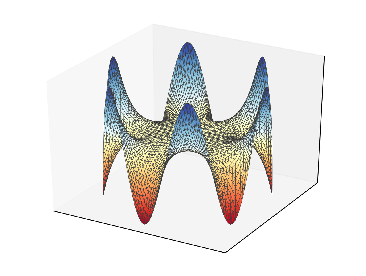
import numpy as np
from numpy import log, arctan2, pi, mean, arctan
from numpy.linalg import norm, solve
import matplotlib.pyplot as plt
from mpl_toolkits.mplot3d import Axes3D
import meshio


  def assem(coords, elems):
      """Assembly matrices for the BEM problem

      Parameters
      ----------
      coords : ndarray, float
          Coordinates for the nodes.
      elems : ndarray, int
          Connectivity for the elements.

      Returns
      -------
      Gmat : ndarray, float
          Influence matrix for the flow.
      Fmat : ndarray, float
          Influence matrix for primary variable.
      """
      nelems = elems.shape[0]
      Gmat = np.zeros((nelems, nelems))
      Fmat = np.zeros((nelems, nelems))
      for ev_cont, elem1 in enumerate(elems):
          for col_cont, elem2 in enumerate(elems):
              pt_col = mean(coords[elem2], axis=0)
              if ev_cont == col_cont:
                  L = norm(coords[elem1[1]] - coords[elem1[0]])
                  Gmat[ev_cont, ev_cont] = - L/(2*pi)*(log(L/2) - 1)
                  Fmat[ev_cont, ev_cont] = - 0.5
              else:
                  Gij, Fij = influence_coeff(elem1, coords, pt_col)
                  Gmat[ev_cont, col_cont] = Gij
                  Fmat[ev_cont, col_cont] = Fij
      return Gmat, Fmat


  def influence_coeff(elem, coords, pt_col):
      """Compute influence coefficients

      Parameters
      ----------
      elems : ndarray, int
          Connectivity for the elements.
      coords : ndarray, float
          Coordinates for the nodes.
      pt_col : ndarray
          Coordinates of the colocation point.

      Returns
      -------
      G_coeff : float
          Influence coefficient for flows.
      F_coeff : float
          Influence coefficient for primary variable.
      """
      dcos = coords[elem[1]] - coords[elem[0]]
      dcos = dcos / norm(dcos)
      rotmat = np.array([[dcos[1], -dcos[0]],
                      [dcos[0], dcos[1]]])
      r_A = rotmat.dot(coords[elem[0]] - pt_col)
      r_B = rotmat.dot(coords[elem[1]] - pt_col)
      theta_A = arctan2(r_A[1], r_A[0])
      theta_B = arctan2(r_B[1], r_B[0])
      if norm(r_A) <= 1e-6:
          G_coeff = r_B[1]*(log(norm(r_B)) - 1) + theta_B*r_B[0]
      elif norm(r_B) <= 1e-6:
          G_coeff = -(r_A[1]*(log(norm(r_A)) - 1) + theta_A*r_A[0])
      else:
          G_coeff = r_B[1]*(log(norm(r_B)) - 1) + theta_B*r_B[0] -\
                  (r_A[1]*(log(norm(r_A)) - 1) + theta_A*r_A[0])
      F_coeff = theta_B - theta_A
      return -G_coeff/(2*pi), F_coeff/(2*pi)


  def eval_sol(ev_coords, coords, elems, u_boundary, q_boundary):
      """Evaluate the solution in a set of points

      Parameters
      ----------
      ev_coords : ndarray, float
          Coordinates of the evaluation points.
      coords : ndarray, float
          Coordinates for the nodes.
      elems : ndarray, int
          Connectivity for the elements.
      u_boundary : ndarray, float
          Primary variable in the nodes.
      q_boundary : [type]
          Flows in the nodes.

      Returns
      -------
      solution : ndarray, float
          Solution evaluated in the given points.
      """
      npts = ev_coords.shape[0]
      solution = np.zeros(npts)
      for k in range(npts):
          for ev_cont, elem in enumerate(elems):
              pt_col = ev_coords[k]
              G, F = influence_coeff(elem, coords, pt_col)
              solution[k] += u_boundary[ev_cont]*F - q_boundary[ev_cont]*G
      return solution


#%% Simulation
mesh = meshio.read("disk.msh")
elems = mesh.cells["line"]
bound_nodes = list(set(elems.flatten()))
coords = mesh.points[bound_nodes, :2]
x, y = coords.T
x_m, y_m = 0.5*(coords[elems[:, 0]] + coords[elems[:, 1]]).T
theta = np.arctan2(y_m, x_m)
u_boundary = 3*np.cos(6*theta)


#%% Assembly
Gmat, Fmat = assem(coords, elems)

#%% Solution
q_boundary = solve(Gmat, Fmat.dot(u_boundary))

#%% Evaluation
ev_coords =  mesh.points[:, :2]
ev_x, ev_y = ev_coords.T
solution = eval_sol(ev_coords, coords, elems, u_boundary, q_boundary)

#%% Visualization
tris = mesh.cells["triangle"]
fig = plt.figure()
ax = fig.add_subplot(111, projection='3d')
ax.plot_trisurf(ev_x, ev_y, solution, cmap="RdYlBu", lw=0.3,
                edgecolor="#3c3c3c")
plt.xticks([])
plt.yticks([])
ax.set_zticks([])
plt.savefig("bem_solution.png", bbox_inches="tight", transparent=True,
            dpi=300)
En este caso obtenemos el siguiente resultado.
Comentarios
Comments powered by Disqus