Using MikTex with LaTeX Workshop on Windows

This is a post to mention how to setup Visual Studio Code for LaTeX—through the LaTeX Workshop extension.

In the past, I have used several text editors and for LaTeX. A couple of years ago I replaced TeXstudio for VS Code, and I think that it works just fine. Visual Studio Code is one of the most used IDE right now. One advantage of using VS Code to type your documents is that you can set it up to fit your workflow and use it for several languages/purposes. It is also cross-platform, you will not be worrying for having different workflows in Linux or Windows.

You need to follow these steps to make it work:

  • Install Perl. You can use Strawberry Perl in Windows.

  • If you don't have administrator privileges you can install the portable version and add the path to the executable to the PATH environment variable.

  • Install MikTeX. The creator of LaTeX Workshop suggests to use TeX Live instead because it already comes with Perl and you could skip one step in this list. The disadvantages of using TeX Live instead of MikTeX are more (see here).

  • Install LaTeX Workshop.

References

  1. Cangemi, Denis. “The Reasons Why You Must Use Visual Studio Code.” Medium, 13 Aug. 2020, https://blog.devgenius.io/the-reasons-why-you-must-use-visual-studio-code-b522f946a849.

  2. Wright, Joseph. “TeX on Windows: TeX Live versus MiKTeX Revisited.” Some TeX Developments, 18 Dec. 2016, https://www.texdev.net/2016/12/18/tex-on-windows-tex-live-versus-miktex-revisited/.


Technical writing: Using Figures

In a previous post I mentioned some general aspects of technical writing. In this one, I would like to talk about including figures in technical documents.

This post is about some details on the planning of figures for technical documents. The main document in mind is a technical article (research paper, techincal report). Although, it also applies to presentations or posters.

Graphic formats

First, I should mention that there are two main types of graphics, namely:

  • vector graphics; and

  • raster graphics.

They serve different purposes and we should use them accordingly. For example, for diagrams or schematics is better to use vector formats, in general. On the other hand, raster formats are better suited for images such as photographs or illustrations.

Vector graphics

A vector image is an image that is made up of geometric entities. In this case, the stored information is not point-to-point but the construction of the shapes that constitute it. For this reason, these images don't pixelate because the information you have is how to build it. This type of images is the best options for schematics and diagrams, since the only stored information are the strokes and text added to them. The de facto standard for this type of images is PDF —it is the one I usually include in my documents \(\LaTeX\). Although PDF is the standard, the preferred format is SVG (Scalable Vector Graphics) which is a standard across the internet and most modern browsers let you render them.

Raster graphics

A raster image is an image which is represented by an array (or rectangular grid) of pixels. In other words, the color information that there are in each point of the image. The most popular formats store the compressed information. For high contrast graphics (such as schematics or diagrams) the best format is PNG. If you have an animation, GIF would be preferable. And in the case of photographs it is better to use JPG.

Summary for formats

Summarizing, we should use JPG images (only) for photographs and SVG for schematics/diagrams. Another attribute that may be useful is the management of layers. Having several layers gives you the option of stacking different types of information separately. For example, you can have the background, the image, and the annotations in different layers. This way you can modify only the part of the figure that concerns you. You can automate the translation of the annotations this way without much problem. Formats such as SVG let you have several layers. In the case of raster formats, we have the option to use TIFF.

Regarding software to generate/edit this type of images I must say that there are a large number of programs that allow exporting to these formats: Python/Matplotlib, Matlab, Inkscape, Adobe Illustrator, GIMP, Photoshop, LibreOffice. If the graph is generated from a calculation or a data series I use Matplotlib. If, instead, we want to make a schematic my tool of choice is Inkscape. This program is intended to be a free alternative to programs like Adobe Illustrator —and it does achieve it. Obviously, you could use Illustrator or Corel Draw for this task. If the only use would be to make technical schematics, I think it would be a waste.

Designing figures for documents

I suggest starting from the nominal size of the figure in the document. For most of our documents, the figures will remain digital and this might seem counterintuitive. Nevertheless, I find this approach much easier. One of the reasons is that we still embed our figure in a document with a nominal size. Also, when thinking about font size it is common that we have as reference printed text. On top of that, we should consider that the human eye has a resolution limit, so we can't just scale down our figures.

Also, there is no such thing as resolution of a digital image. Resolution refers to a density of pixels per unit length. This makes sense when printing images, but not in the digital case. Nevertheless, the figures have a nominal size and hence a nominal resolution. That is, the number of pixels in one direction divided by its nominal size. It is a good idea to consider a minimal resolution of 150 dpi (dots per inch). For example, an image of 6 in × 3 in. This image would have a size of (at 150 dpi) of de 900 px × 450 px.

The following Python snippet creates a figure of size 6 in × 3 in, and plots the function \(f(x) = \sin(x^2)\) and stores it as an image of size 900 in × 450 in.

import numpy as np
import matplotlib.pyplot as plt
x = np.linspace(0, 2*np.pi, 500, linewidth=2)
y = np.sin(x**2)
plt.figure(figsize=(6, 3))
plt.plot(x, y)
plt.xlabel("x", fontsize=10)
plt.ylabel("y", fontsize=10)
plt.savefig("fig_ex_python.png", dpi)

And the following in Matlab.

fig = figure(1);
fig.Units = 'inches';
fig.Position(3:4) =  [6 4];
x = linspace(0, 2*pi, 500);
y = sin(x.^2);
plot(x, y, 'LineWidth', 2);
xlabel('x', 'FontSize', 10)
ylabel('y', 'FontSize', 10)
set(fig, 'PaperSize', [6,4]);
print(fig,'fig_ex_matlab', '-dpng', '-r150');

Following I summarize some sizes for articles, posters and slides.

Articles

For an article is common to use letter size that is 8.5 in × 11 in (215.9 mm × 279.4 mm). Another common size is A4 that is 210 mm × 297 mm (8.27 in × 11.7 in).

A guideline for common sizes is the following:

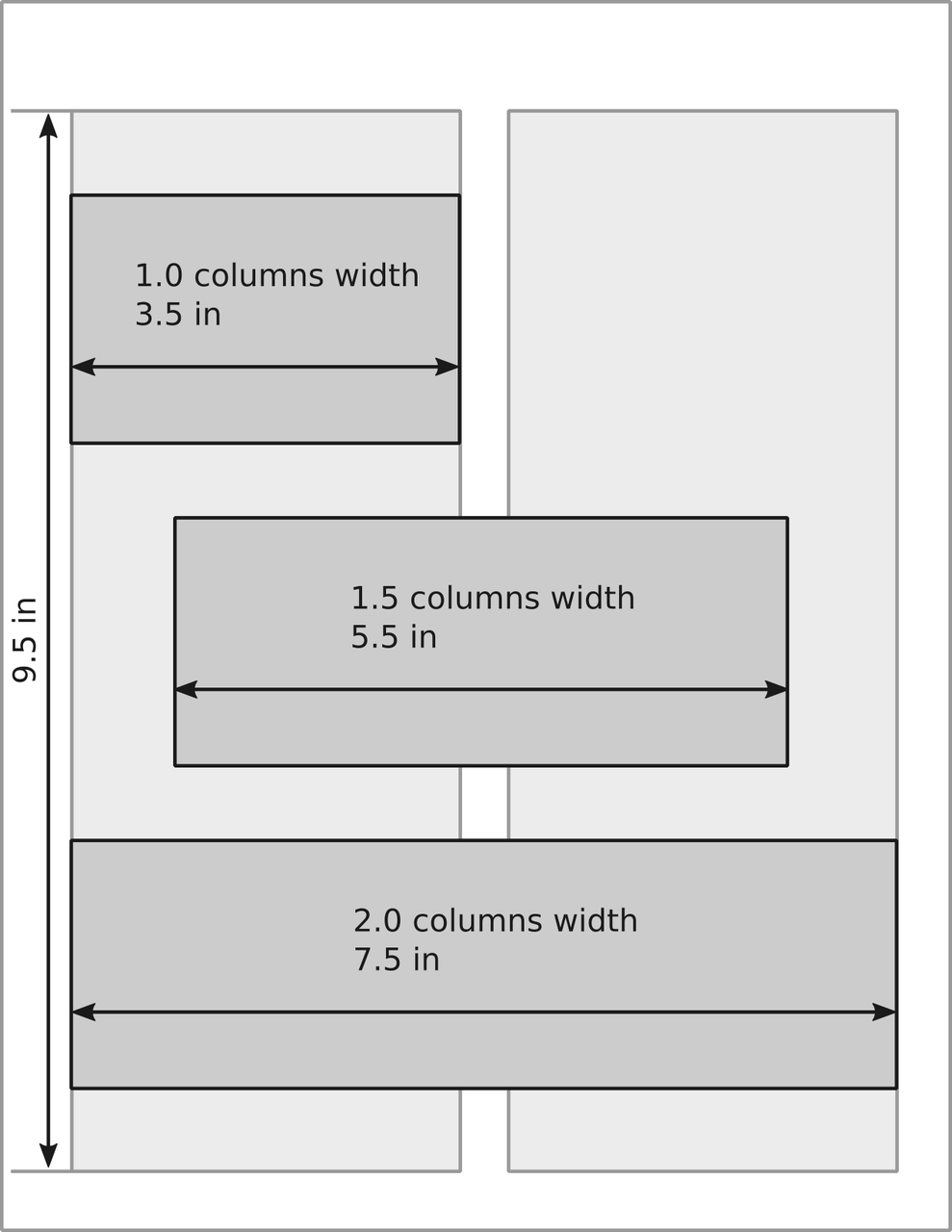
  • 1.0 columns width: 90 mm (3.5 in);

  • 1.5 columns width: 140 mm (5.5 in);

  • 2.0 columns width: 190 mm (6.5 in);

and depicted in the following image.

Figure widths compared with letter size paper.

If we consider a resolution of 300 dpi, we have the following number of pixels horizontally

  • 1.0 columns width: 1050 pixels;

  • 1.5 columns width: 1650 pixels; and

  • 2.0 columns width: 1950 pixels.

Note that an HD display has 1920 pixels in the horizontal direction. That means that you need a HD display to be able to see that much pixels.

Regarding text size, it is common to have sizes between 8 and 12 pts for figures.

Posters

In the case of an A0 size paper (841 mm × 1189 mm, 33 in × 47 in) the sizes would be around:

  • 1.0 columns width: 360 mm (14 in);

  • 1.5 columns width: 560 mm (22 in); and

  • 2.0 columns width: 760 mm (26 in).

Keep in mind that a poster might not fit into the two-column format. Although, I still find the reference for the size useful.

Regarding the size of fonts in posters it is a good idea to keep it over 24 pts (see reference 3).

Slides

In the case of slides there are two common aspect ratios 16:9 and 4:3. And, different software have different nominal sizes. The following table present the nominal sizes for LibreOffice Impress and MS Power Point.

16:9

4:3

LibreOffice Impress

11.02 in × 6.20 in

11.02 in × 8.00 in

MS Power Point

13.32 in × 7.50 in

10.00 in × 7.50 in

References

  1. Matthew Butterick (2019). Butterick's Practical Typography. Second edition, Matthew Butterick.

  2. Rougier, Nicolas P., Michael Droettboom, and Philip E. Bourne (2014). “Ten Simple Rules for Better Figures.” PLOS Computational Biology 10(9):e1003833. DOI: 10.1371/journal.pcbi.1003833.

  3. Erren, Thomas C., and Philip E. Bourne. 2007. “Ten Simple Rules for a Good Poster Presentation.” PLOS Computational Biology 3(5):e102. DOI: 10.1371/journal.pcbi.0030102

  4. Elsevier. (n.d.). "Artwork Overview." Retrieved November 1, 2021, from https://www.elsevier.com/authors/policies-and-guidelines/artwork-and-media-instructions/artwork-overview

  5. Elsevier. (n.d.). "Artwork sizing." Retrieved November 1, 2021, from https://www.elsevier.com/authors/policies-and-guidelines/artwork-and-media-instructions/artwork-sizing

  6. Journal of applied physics (n.d.). "Preparing Your Manuscript: Authors Instruction." Retrieved November 1, 2021, from https://aip.scitation.org/jap/authors/manuscript


How much chicharrón can Jeff Bezos buy?

This is a calculation made by Sebastián Tobón when he was taking the course Numerical Methods for Partial Differential Equations (in 2020). The purpose was to encourage doing quick calculations (back-of-the-envelope) and having the size of some numbers (for example, 10¹²) in their heads. Here is the question I asked:

How much chicharrón (pork rinds) can Jeff Bezos buy?

Below is his answer.

Sebastián's answer

Suppose an average pig weighs 80 kg. If its muscle tissue constitutes 35% to 40% of its body weight, we can ge 30 kg of meat.

Jeff Bezos has a net worth of

\begin{equation*} JB = 115.7 \times 10^9 \text{ USD}\, . \end{equation*}

The price of 100 g of chicharrón is

\begin{equation*} 7000\text{ COP}\, \frac{1\text{ USD}}{3539.13\text{ COP}} = 1.978\text{ USD}\, . \end{equation*}

Jeff Bezos can therefore buy

\begin{equation*} \frac{115.7\times 10^9\text{ USD}}{\frac{1.978\text{ USD}}{100\text{ g}}} = 5.85\times 10^{12}\text{ g of chicharrón.} \end{equation*}

The total number of pigs in the world is 1×10⁹. This is equivalent to a total of

\begin{equation*} 1\times 10^9 \text{ heads} \times \frac{30\text{ kg}}{1\text{ head}} = 3\times 10^{13} \text{ g of chicharrón.} \end{equation*}

In order to buy all the pork rinds in the world, he must increase his net worth by 5.13.

The most expensive pigs in the world cost around 1000 USD, then

\begin{equation*} \frac{1000\text{ USD}}{\text{head}}\times 10^9\text{ heads} = 10^{12}\text{ USD}\, . \end{equation*}

On the other hand, he can buy 5.85 times the amount of pigs globally — the most expensive in the market. Therefore

it is more profitable for him to buy all the pigs in the world.


Using Wolfram Language in Jupyter: A free alternative to Mathematica

In this post I am going to describe how to add the Wolfram Language to the Jupyter notebook. This provides a free alternative to Mathematica with, pretty much, the same syntax. The use of the Wolfram Engine is free for non-production as described in their website:

The Free Wolfram Engine for Developers is available for non-production software development.

You can use this product to:

  • develop a product for yourself or your company

  • conduct personal projects at home, at school, at work

  • explore the Wolfram Language for future production projects

Installation

To install you should do the following steps:

  • Download Wolfram Engine.

  • Create a Wolfram account, if you don't have one.

  • Execute the installer.

  • Type the following in a terminal

wolframscript

and you should be asked for your email and password.

After that you should be in a terminal and see the following

Wolfram Engine activated. See https://www.wolfram.com/wolframscript/ for more information.
Wolfram Language 12.2.0 Engine for Linux x86 (64-bit)
Copyright 1988-2021 Wolfram Research, Inc.

And we can try that it is working

In[1]:= $Version

Out[1]= 12.2.0 for Linux x86 (64-bit) (January 7, 2021)

In[2]:= Integrate[1/(1 + x^2), x]

Out[2]= ArcTan[x]

Now we need to install WolframLanguageForJupyter. For that we can type the following in a terminal

git clone https://github.com/WolframResearch/WolframLanguageForJupyter.git

cd WolframLanguageForJupyter/

./configure-jupyter.wls add

To test that it is installed we can type the following in a terminal

jupyter kernelspec list

and it should have an output that includes a line similar to the following

wolframlanguage12.   /home/nicoguaro/.local/share/jupyter/kernels/wolframlanguage12.2

Or we could also try with

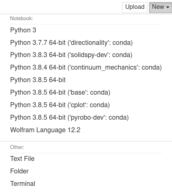
jupyter notebook

and see the following in the kernel menu.

Kernel menu after installing WolframLanguageForJupyter.

Test drive

I tested some of the capabilities and you can download the notebook or see a static version here.

Let's compute the integral

\begin{equation*} \int \frac{1}{1 + x^3}\mathrm{d}x\, . \end{equation*}
sol:= Integrate[1/(1 + x^3), x]
TeXForm[sol]
\begin{equation*} -\frac{1}{6} \log \left(x^2-x+1\right)+\frac{1}{3} \log (x+1)+\frac{\tan^{-1}\left(\frac{2 x-1}{\sqrt{3}}\right)}{\sqrt{3}} \end{equation*}

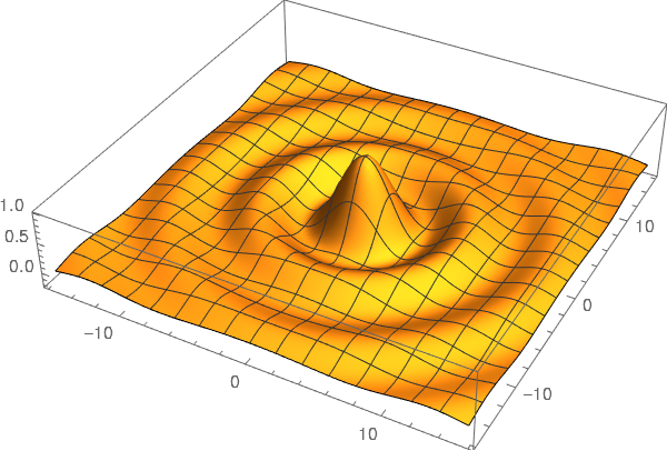
And make a 3D plot.

fun:= Sin[Sqrt[x^2 + y^2]]/Sqrt[x^2 + y^2]
Plot3D[fun, {x, -5*Pi, 5*Pi}, {y, -5*Pi, 5*Pi},
    PlotPoints -> 100, BoxRatios -> {1, 1, 0.2},
    PlotRange -> All]
3D plot in the notebook.

In this case we don't have an interactive image. This is still not implemented, but if you are interested there is an open issue about it in GitHub.

Coming back to the Boundary element method

During October (2017) I wrote a program per day for some well-known numerical methods in both Python and Julia. It was intended to be an exercise to learn some Julia. You can see a summary here. I succeeded in 30 of the challenges, except for the BEM (Boundary Element Method), where I could not figure out what was wrong that day. The original post is here.

Thomas Klimpel found the mistake and wrote an email where he described my mistakes. So, I am creating a new post with a correct implementation of the BEM.

The Boundary Element Method

We want so solve the equation

\begin{equation*} \nabla^2 u = -f(x, y)\quad \forall (x, y) \in \Omega\, , \end{equation*}

with

\begin{equation*} u(x) = g(x, y), \quad \forall (x, y)\in \partial \Omega \, . \end{equation*}

For this method, we need to use an integral representation of the equation, that, in this case, is

\begin{equation*} u(\boldsymbol{\xi}) = \int_{S} [u(\mathbf{x}) F(\mathbf{x}, \boldsymbol{\xi}) - q(\mathbf{x})G(\mathbf{x}, \boldsymbol{\xi})]\mathrm{d}S(\mathbf{x}) + \int_{V} f(\mathbf{x}) G(\mathbf{x}, \boldsymbol{\xi}) \mathrm{d}V(\mathbf{x}) \end{equation*}

with

\begin{equation*} G(\mathbf{x}, \boldsymbol{\xi})= -\frac{1}{2\pi}\ln|\mathbf{x} - \xi| \end{equation*}

and

\begin{equation*} F(\mathbf{x}, \boldsymbol{\xi}) = -\frac{1}{2\pi |\mathbf{x} - \boldsymbol{\xi}|^2} (\mathbf{x} - \boldsymbol{\xi})\cdot\hat{\mathbf{n}} \end{equation*}

Then, we can form a system of equations

\begin{equation*} [G]\{q\} = [F]\{u\}\, , \end{equation*}

that we obtain by discretization of the boundary. If we take constant variables over the discretization, the integral can be computed analytically by

\begin{equation*} G_{nm} = -\frac{1}{2\pi}\left[r \sin\theta\left(\ln|r| - 1\right) + \theta r\cos\theta\right]^{\theta_B, r_B}_{\theta_A, r_A} \end{equation*}

and

\begin{equation*} F_{nm} = \left[\frac{\theta}{2\pi}\right]^{\theta_B}_{\theta_A} \end{equation*}

for points \(n\) and \(m\) in different elements, and the subindices \(A,B\) refer to the endpoints of the evaluation element. We should be careful evaluating this expression since both \(r_A\) and \(r_B\) can be (close to) zero and make it explode. Also, here it was the main problem since I forgot to compute the angles with respect to elements that are, in general, not aligned with horizontal or vertical axes.

For diagonal terms the integrals evaluate to

\begin{equation*} G_{nn} = -\frac{L}{2\pi}\left(\ln\left\vert\frac{L}{2}\right\vert - 1\right) \end{equation*}

and

\begin{equation*} F_{nn} = - \frac{1}{2} \end{equation*}

with \(L\) the size of the element.

Following is the code. Keep in mind that this code works for purely Dirichlet problems. For mixed Dirichlet-Neumann the influence matrices would need rearranging to separate known and unknowns in opposite sides of the equation.

You can download the files for this project here. It includes a YML file to create a conda environment with the dependencies listed. For example, it uses version 3.0 of Meshio.

import numpy as np
from numpy import log, arctan2, pi, mean, arctan
from numpy.linalg import norm, solve
import matplotlib.pyplot as plt
from mpl_toolkits.mplot3d import Axes3D
import meshio


  def assem(coords, elems):
      """Assembly matrices for the BEM problem

      Parameters
      ----------
      coords : ndarray, float
          Coordinates for the nodes.
      elems : ndarray, int
          Connectivity for the elements.

      Returns
      -------
      Gmat : ndarray, float
          Influence matrix for the flow.
      Fmat : ndarray, float
          Influence matrix for primary variable.
      """
      nelems = elems.shape[0]
      Gmat = np.zeros((nelems, nelems))
      Fmat = np.zeros((nelems, nelems))
      for ev_cont, elem1 in enumerate(elems):
          for col_cont, elem2 in enumerate(elems):
              pt_col = mean(coords[elem2], axis=0)
              if ev_cont == col_cont:
                  L = norm(coords[elem1[1]] - coords[elem1[0]])
                  Gmat[ev_cont, ev_cont] = - L/(2*pi)*(log(L/2) - 1)
                  Fmat[ev_cont, ev_cont] = - 0.5
              else:
                  Gij, Fij = influence_coeff(elem1, coords, pt_col)
                  Gmat[ev_cont, col_cont] = Gij
                  Fmat[ev_cont, col_cont] = Fij
      return Gmat, Fmat


  def influence_coeff(elem, coords, pt_col):
      """Compute influence coefficients

      Parameters
      ----------
      elems : ndarray, int
          Connectivity for the elements.
      coords : ndarray, float
          Coordinates for the nodes.
      pt_col : ndarray
          Coordinates of the colocation point.

      Returns
      -------
      G_coeff : float
          Influence coefficient for flows.
      F_coeff : float
          Influence coefficient for primary variable.
      """
      dcos = coords[elem[1]] - coords[elem[0]]
      dcos = dcos / norm(dcos)
      rotmat = np.array([[dcos[1], -dcos[0]],
                      [dcos[0], dcos[1]]])
      r_A = rotmat.dot(coords[elem[0]] - pt_col)
      r_B = rotmat.dot(coords[elem[1]] - pt_col)
      theta_A = arctan2(r_A[1], r_A[0])
      theta_B = arctan2(r_B[1], r_B[0])
      if norm(r_A) <= 1e-6:
          G_coeff = r_B[1]*(log(norm(r_B)) - 1) + theta_B*r_B[0]
      elif norm(r_B) <= 1e-6:
          G_coeff = -(r_A[1]*(log(norm(r_A)) - 1) + theta_A*r_A[0])
      else:
          G_coeff = r_B[1]*(log(norm(r_B)) - 1) + theta_B*r_B[0] -\
                  (r_A[1]*(log(norm(r_A)) - 1) + theta_A*r_A[0])
      F_coeff = theta_B - theta_A
      return -G_coeff/(2*pi), F_coeff/(2*pi)


  def eval_sol(ev_coords, coords, elems, u_boundary, q_boundary):
      """Evaluate the solution in a set of points

      Parameters
      ----------
      ev_coords : ndarray, float
          Coordinates of the evaluation points.
      coords : ndarray, float
          Coordinates for the nodes.
      elems : ndarray, int
          Connectivity for the elements.
      u_boundary : ndarray, float
          Primary variable in the nodes.
      q_boundary : [type]
          Flows in the nodes.

      Returns
      -------
      solution : ndarray, float
          Solution evaluated in the given points.
      """
      npts = ev_coords.shape[0]
      solution = np.zeros(npts)
      for k in range(npts):
          for ev_cont, elem in enumerate(elems):
              pt_col = ev_coords[k]
              G, F = influence_coeff(elem, coords, pt_col)
              solution[k] += u_boundary[ev_cont]*F - q_boundary[ev_cont]*G
      return solution


#%% Simulation
mesh = meshio.read("disk.msh")
elems = mesh.cells["line"]
bound_nodes = list(set(elems.flatten()))
coords = mesh.points[bound_nodes, :2]
x, y = coords.T
x_m, y_m = 0.5*(coords[elems[:, 0]] + coords[elems[:, 1]]).T
theta = np.arctan2(y_m, x_m)
u_boundary = 3*np.cos(6*theta)


#%% Assembly
Gmat, Fmat = assem(coords, elems)

#%% Solution
q_boundary = solve(Gmat, Fmat.dot(u_boundary))

#%% Evaluation
ev_coords =  mesh.points[:, :2]
ev_x, ev_y = ev_coords.T
solution = eval_sol(ev_coords, coords, elems, u_boundary, q_boundary)

#%% Visualization
tris = mesh.cells["triangle"]
fig = plt.figure()
ax = fig.add_subplot(111, projection='3d')
ax.plot_trisurf(ev_x, ev_y, solution, cmap="RdYlBu", lw=0.3,
                edgecolor="#3c3c3c")
plt.xticks([])
plt.yticks([])
ax.set_zticks([])
plt.savefig("bem_solution.png", bbox_inches="tight", transparent=True,
            dpi=300)

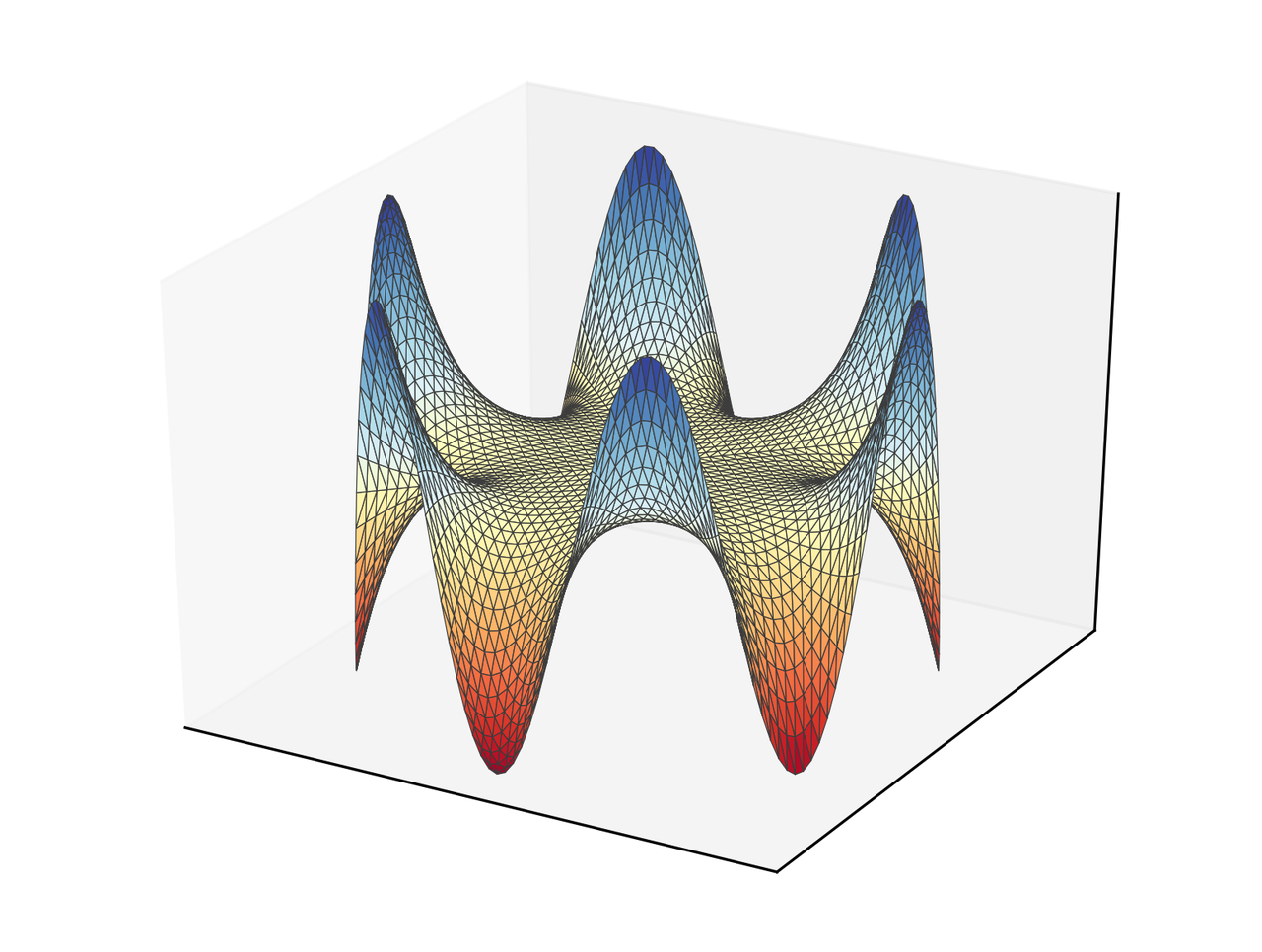
The result in this case is the following.

Solution of the differential equation using the BEM.

Downloading videos from MS Stream

This week a student asked me about downloading the videos from one of the courses from MS Stream. The problem is that if you are not a proprietary of the video you cannot download it. So, I will show you an option to download videos without being a proprietary of them.

Disclaimer: It might be a good idea if you ask your organization about the copyright of the videos.

Prerequisites

You will need the following:

destreamer installation

After getting the prerequisites you can download destreamer using

$ git clone https://github.com/snobu/destreamer
$ cd destreamer
$ npm install
$ npm run build

in a terminal.

If you do not want to play with environment variables, I suggest that you just add ffmpeg to the same folder as destreamer.

Downloading

After that, you need to navigate to the folder where you downloaded destreamer and

$ ./destreamer.sh -i "https://web.microsoftstream.com/video/VIDEO_ID"

in Mac or Linux,

$ destreamer.cmd -i "https://web.microsoftstream.com/video/VIDEO_ID"

in the command prompt in Windows, and

$ destreamer.ps1 -i "https://web.microsoftstream.com/video/VIDEO_ID"

in PowerShell.``VIDEO_ID`` refers to the identifier in MS Stream.

If you want to download several files (like a complete course), you can create a file with the URLs and use

$ destreamer.cmd -f filename.txt

Randomized Marking of a Tetrahedron

Yesterday (June 4, 2020), Christian Howard posted on Twitter the following question

You are given a tetrahedron τ. For each triangular facet of τ, we uniformly at random mark one of their edges. What is the probability that there exists an edge of τ that is marked twice?

I thought about a little bit but I couldn't find how to count properly. Then, a number popped up in my mind out of the blue: \(2/3\), but I don't know why. So, I decided to run a simulation to check this number.

The right answer is \(51/81\) that is approximately 63%. This calculation is well explained in Christian's blog and with some cool drawings (and memes).

The algorithm

The algorithm is quite simple. I number the edges in each face following a counter-clockwise orientation:

  • face 0: edge 0, edge 1, edge 2

  • face 1: edge 0, edge 3, edge 4

  • face 2: edge 1, edge 5, edge 3

  • face 3: edge 2, edge 4, edge 5

Then, I take each face and pick a random number from \((0, 1, 2)\) and mark the corresponding edge, and move to the following face. I repeat this process several times and I count the favorable cases and divide them by the number of trials to get an estimate of the probability.

Following is a Python code that follows this idea.

import numpy as np
import matplotlib.pyplot as plt

faces = np.array([
        [0, 1, 2],
        [0, 3, 4],
        [1, 5, 3],
        [2, 4, 5]])


def mark_edges():
    marked_edges = np.zeros((6), dtype=int)
    for face in faces:
        num = np.random.randint(0, 3)
        edge = face[num]
        marked_edges[edge] += 1
    return marked_edges


def comp_probs(N_min=1, N_max=5, ntrials=100):
    prob = []
    N_vals = np.logspace(N_min, N_max, ntrials, dtype=int)
    for N in N_vals:
        cont_marked = 0
        for cont in range(N):
            marked = mark_edges()
            if 2 in marked:
                cont_marked += 1
        prob.append(cont_marked/N)
    return N_vals, prob


#%% Computation
N_min = 1
N_max = 5
ntrials = 100
np.random.seed(seed=2)
N_vals, prob = comp_probs(N_min, N_max, ntrials)

#%% Plotting
plt.figure(figsize=(4, 3))
plt.hlines(0.63, 10**N_min, 10**N_max, color="#3f3f3f")
plt.semilogx(N_vals, np.array(prob), "o", alpha=0.5)
plt.xlabel("Number of trials")
plt.ylabel("Estimated probability")
plt.savefig("prob_tet.svg", dpi=300, bbox_inches="tight")
plt.show()

And we can see the following evolution for different number of trials.

Estimated probabilities for different sample sizes.

Technical writing

This is the first post about technical writing [*] from a series that I will be creating and uploading. Technical writing is something that most of us have to deal with in different contexts. For example, in college coursework, research publications, software documentation. The main idea of the series is to mention some of the tricks that I have learned over the years and some tools that might come in handy.

Future posts will (probably) be about:

The current post

As mentioned above, technical writing is something that a lot of persons have to deal with. This is a skill that is sometimes overlooked, but it should not. According to the U.S. Bureau of Labor Statistics

Technical writers prepare instruction manuals, how-to guides, journal articles, and other supporting documents to communicate complex and technical information more easily.

And it is a desired skill in the workplace. Its demand is expected to grow around 10% in the current decade.

Typography

The first thing that I should mention is that writing documents is typography. "Putting documents" together is typography because we are designing with text (Butterick, 2019). So, we should consider ourselves typographers since we are constantly designing documents.

I would suggest taking a look at "Butterick's Practical Typography" since it is a really good book about it and it reads smoothly. I will mention some important points here according to Butterick's "Typography in ten minutes":

  1. The most important typographic selection is on the body text. This is due to the fact that it is most of the document.

  2. Choose a point size between 10-12 points for printed documents and 15-25 pixels for digital documents.

  3. Line spacing should be between 120-145 % of the point size.

  4. Line length should be between 45-90 characters. This is roughly 2 or 3 small caps alphabets:

    abcdefghijklmnopqrstuvwxyzabcdefghijklmnopqrstuvwxyzabcd

  5. Mind the selection of your font. Try to avoid default fonts such as Arial, Calibri or Times New Roman.

Editors

Another point that I want to touch in this post is about editors. The first question that arises is "what editor should I use?". The short answer is: use whatever your peers are using. That's my best advice; that way you have people to discuss with you about your doubts.

The long answer … is that each editor has its weak and strong points. I have written scientific papers in LaTeX, LibreOffice Writer and MS Word; all of them look professional. So, in the end, you can write your documents in several ways and achieve a similar result. I prefer to use LaTeX for long documents since it is centered in the structure of the document instead of the appearance and this is the way one should manage a long document like a dissertation, in my opinion.

If you just want me to pick one editor and suggest it to you, I would say that you should ride with LibreOffice. A good reference for it is "Designing with LibreOffice". Once you learn how to use styles you will ask how have you been writing documents all this time.

There are two main flavors for editors that I am going to discuss: WYSIWYG (What You See Is What You Get) and markup-based editors.

  • WYSIWYG. This category is the one that most people is familiar with. Two examples are:

    • LibreOffice writer; and

    • Microsoft Word.

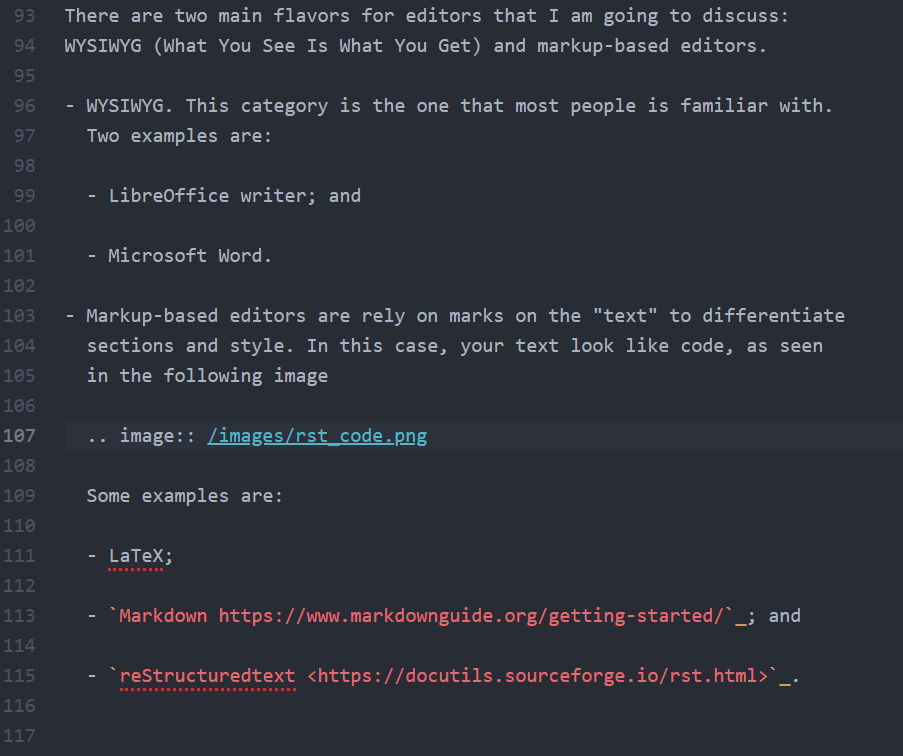
  • Markup-based editors rely on marks on the "text" to differentiate sections and styles. In this case, your text looks like code, as seen in the following image

    /images/rst_code.png

    Some examples are:

Independently of what your main editor is I suggest that you use Pandoc. It allows you to convert between several formats, making the process a little bit easier. There is even an editor based completely on it named Panwriter.

References

  1. Matthew Butterick (2019). Butterick's Practical Typography. Second edition, Matthew Butterick.

  2. Wikibooks contributors. (2020). LaTeX. Wikibooks, The Free Textbook Project.

  3. Bruce Byfield (2016). Designing with LibreOffice. Friends of OpenDocument, Inc.

  4. Deville, S. (2015). Writing academic papers in plain text with Markdown and Jupyter notebook. Sylvain Deville.

  5. Eric Holscher (2016). An introduction to Sphinx and Read the Docs for Technical Writers.

Technical writing: using math

In a previous post I mentioned some general aspects of technical writing. In this one, I would like to talk about including mathematical expressions in technical documents.

There are two main ways to include math in your documents:

  • using text; and

  • using a graphic interface.

Using a graphic interface, such as the equation editor in LibreOffice Writer or MS Word, or MathType is convenient. You don't need to memorize anything and you can look at your expressions while creating them. Nevertheless, it can be slow compared to using text input — once you are comfortable with the syntax.

There are two main flavors of equations used over the internet:

  • MathML is a W3C standard for equations and it is included in HTML5, so it would work in all modern browsers. The problem with it is that it is not designed to be written by hand. So one can use it if have some automatic way of generating the code.

  • LaTeX is my suggested way to write equations. The learning curve might be a little bit steep at the beginning but it pays off.

One tool that helps with equations is MathPix Snip that automatically generates LaTeX or MathML code from an image, even a handwritten one. Another tool that is really useful is Detexify that let you draw a symbol and gives you the LaTeX syntax for it.

In the remaining of the posts I will show my suggestions for working with equations in LibreOffice and MS Word. If you are using LaTeX or MarkDown/ReStructuredText for your documents you are already using LaTeX for your equations.

LibreOffice

LibreOffice has its own math editor with its own syntax and it works fine for small expressions, but it gets complicated for large equations or long algebraic manipulations. For LibreOffice I would suggest to use TexMaths, it is simple to use and works for the word processor (Writer) and presentations (Impress). I suppose it also works for spreadsheets (Calc), but I don't remember using equations in one.

MS Office

MS Office has its own math editor as well, it works fine and is easy to use. Nevertheless, the same problem appears when you want long expressions. One option is to directly use LaTeX in Office but I prefer to use IguanaTex. It is a complement that allows to input equations similarly to TexMaths in LibreOffice.

You could also directly paste MathML equations into MS Word (>2013 and Windows).

Use a SymPy

Indepent of the tool that you use to write your documents I strongly suggest to use a CAS (Computer Algebra System), such as Mathematica or SymPy. These programs have automatic generation of LaTeX and MathML from expression and that can ease the process a lot.

Let's check an example. Suppose that we have the function

\begin{equation*} f(x) = \exp(-x^2) \sin(3*x) \end{equation*}

and we want to compute its second derivative

\begin{equation*} f''(x) = \left(- 12 x \cos{\left(3 x \right)} + 2 \left(2 x^{2} - 1\right) \sin{\left(3 x \right)} - 9 \sin{\left(3 x \right)}\right) e^{- x^{2}} \end{equation*}

The following code gives us the LaTex code

from sympy import *
init_session()
f = exp(-x**2)*sin(3*x)
fxx = diff(f, x, 2)
print(latex(fxx))

that is

\left(- 12 x \cos{\left(3 x \right)} + 2 \left(2 x^{2} - 1\right) \sin{\left(3 x \right)} - 9 \sin{\left(3 x \right)}\right) e^{- x^{2}}

That corresponds to the code that I used above to render the equation

If, we wanted the MathML code of that expression we could use the following snippet

from sympy import *
init_session()
f = exp(-x**2)*sin(3*x)
fxx = diff(f, x, 2)
print(mathml(fxx, printer="presentation"))

notice the extra argument printer="presentation". If we want to add this to MS Word, for example, we could add the output (that I will not show because is really long) inside the following

<math xmlns = "http://www.w3.org/1998/Math/MathML">
</math>

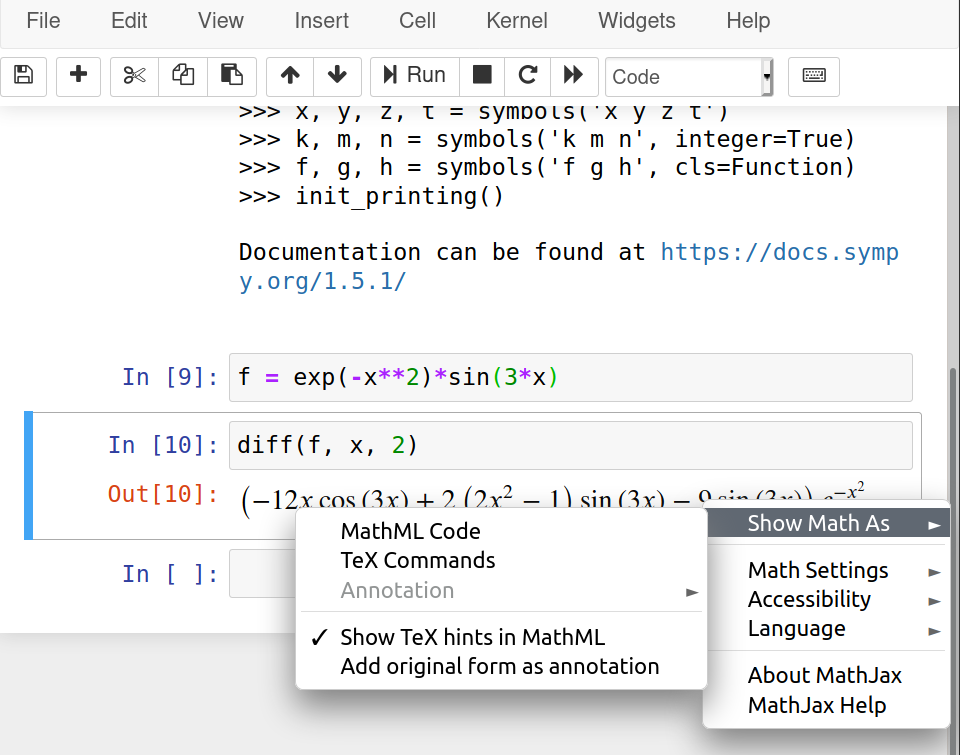
When using Jupyter Notebook this can be done graphically with a right click over the expression. Then, the following menu is shown

/images/jupyter_export_eqs.png

References

  1. “How to Insert Equations in Microsoft Word.” WikiHow, https://www.wikihow.com/Insert-Equations-in-Microsoft-Word. Accessed 3 Aug. 2020.

  2. “Copy MathML into Word to Use as Equation.” Stack Overflow, https://stackoverflow.com/questions/25430775/copy-mathml-into-word-to-use-as-equation. Accessed 3 Aug. 2020.

  3. “Python - Output Sympy Equation to Word Using Mathml.” Stack Overflow, https://stackoverflow.com/questions/40921128/output-sympy-equation-to-word-using-mathml. Accessed 3 Aug. 2020.

  4. OERPUB (2016), “Mathconverter”, https://github.com/oerpub/mathconverter, Accesed 3 Aug. 2020.

Spell Check in Jupyter Notebook

The purpose of this post is to show how to have automatic spell check in Jupyter Notebook, as shown below.

Example of spell checking in Jupyter Notebook.

There are several ways to do this. However, the easiest way is through the (nbextension) Spellchecker. plugin.

Step by step

The steps to follow are those:

  1. Install Jupyter notebook extensions (nbextensions). This includes Spellchecker.

  2. Locate the dictionaries in the folder where the plugin is. Dictionaries must use UTF-8 encoding.

  3. Configure the path of the dictionaries. This can be a URL or a path relative to the folder where the plugin is located.

We will describe each step in detail below.

Step 1: Install nbextensions

There is a list of plugins that add some commonly used functionality to the Jupyter notebook.

Type the following in a terminal, to install it using PIP.

pip install jupyter_contrib_nbextensions

However, if Anaconda is being used the recommended method is to use conda, as shown below.

conda install -c conda-forge jupyter_contrib_nbextensions

This should install the plugins and also the configuration interface. In the main menu of Jupyter notebook a new tab named Nbextension will appear. Here you can choose the add-ons to use. The appearance is as follows.

Graphical interface for Jupyter plugins.

Some recommended plugins are:

  • Collapsible Headings: that allows to hide sections of the documents.

  • RISE: that turns notebooks into presentations.

Step 2: Dictionaries for Spanish

The documentation of Spellchecker suggests using a Python script to download dictionaries from project Chromium. However, these are encoded in ISO-8859-1 (western) and it fails for characters with accents or tildes. So, to avoid problems the dictionary must be UTF-8. They can be downloaded at this link.

Once you have the dictionaries, they must be located in the path of the plugin. On my computer this would be

~/.local/share/jupyter/nbextensions/spellchecker/

and within this we will place them in

~/.local/share/jupyter/nbextensions/spellchecker/typo/dictionaries

This location is arbitrary, the important thing is that we need to know the relative path to the plugin.

Step 3: Plugin Configuration

Now, in the Nbextensions tab we select the plugin and fill the fields with the information from our dictionary:

  • language code to use with typo.js: es_ES

  • url for the dictionary .dic file to use: ./typo/dictionaries/es_ES.dic

  • url for the dictionary .aff file to use: ./typo/dictionaries/es_ES.aff

This is shown below.

Configuration with local files.

Another option is to use the URL for the files. The dictionaries of the project hunspell in UTF-8 are available at https://github.com/wooorm/dictionaries. In this case, the configuration would be:

  • language code to use with typo.js: es_ES

  • url for the dictionary .dic file to use: https://raw.githubusercontent.com/wooorm/dictionaries/master/dictionaries/es/index.dic

  • url for the dictionary .aff file to use: https://raw.githubusercontent.com/wooorm/dictionaries/master/dictionaries/es/index.aff

And it is shown below.

Configuration with remote files.