In this post, we find the Hermite interpolation functions for the
domain [-1, 1]. And then, we use it for a pieciwise interpolation. Notice
that this interpolation has \(C^1\) continuity compared to the
\(C^0\) continuity that is common in Lagrange interpolation.
To compute the polynomials explicitly we use sympy.
from __future__ import division
import numpy as np
import sympy as sym
import matplotlib.pyplot as plt
We want to find a set of basis function that satisfy the following
\begin{align*}
N_1(x_1) &= 1\\
N_1(x_2) &= 0\\
N_2(x_1) &= 1\\
N_2(x_2) &= 0\\
N'_3(x_1) &= 1\\
N'_3(x_2) &= 0\\
N'_4(x_1) &= 1\\
N'_4(x_2) &= 0
\end{align*}
These can be written as
\begin{equation*}
\begin{bmatrix}
1 &x_1 &x_1^2 &x_1^3\\
1 &x_2 &x_2^2 &x_2^3\\
0 &1 &2x_1 &3x_1^2\\
0 &1 &2x_2 &3x_2^2
\end{bmatrix}
\begin{bmatrix}
a_{11} &a_{12} &a_{13} &a_{14}\\
a_{21} &a_{22} &a_{23} &a_{24}\\
a_{31} &a_{32} &a_{33} &a_{34}\\
a_{41} &a_{42} &a_{43} &a_{44}
\end{bmatrix} =
\begin{bmatrix}
1 &0 &0 &0\\
0 &1 &0 &0\\
0 &0 &1 &0\\
0 &0 &0 &1
\end{bmatrix}
\end{equation*}
The formula for interpolation would be
\begin{equation*}
f(x) \approx N_1(x) u_1 + N_2(x) u_2 + |J|(N_3(x) u'_3 + N_4(x) u'_4)\quad \forall x\in [a, b]
\end{equation*}
with \(|J| = (b - a)/2\) the Jacobian determinant of the
transformation.
x1, x2, x = sym.symbols("x1 x2 x")
V = sym.Matrix([
    [1, x1, x1**2, x1**3],
    [1, x2, x2**2, x2**3],
    [0, 1, 2*x1, 3*x1**2],
    [0, 1, 2*x2, 3*x2**2]])
V
\begin{equation*}
\left[\begin{matrix}1 & x_{1} & x_{1}^{2} & x_{1}^{3}\\
1 & x_{2} & x_{2}^{2} & x_{2}^{3}\\
0 & 1 & 2 x_{1} & 3 x_{1}^{2}\\
0 & 1 & 2 x_{2} & 3 x_{2}^{2}\end{matrix}\right]
\end{equation*}
We can see that the previous matrix is a confluent Vandermonder matrix .
It is similar to a Vandermonde matrix for the first \(n\) nodes
and the derivatives of each row for the following ones.
The coefficients for our polynomials are given by the inverse of this matrix.
\begin{equation*}
\left[\begin{matrix}\frac{x_{2}^{2} \left(3 x_{1} - x_{2}\right)}{x_{1}^{3} - 3 x_{1}^{2} x_{2} + 3 x_{1} x_{2}^{2} - x_{2}^{3}} & \frac{x_{1}^{2} \left(x_{1} - 3 x_{2}\right)}{x_{1}^{3} - 3 x_{1}^{2} x_{2} + 3 x_{1} x_{2}^{2} - x_{2}^{3}} & - \frac{x_{1} x_{2}^{2}}{x_{1}^{2} - 2 x_{1} x_{2} + x_{2}^{2}} & - \frac{x_{1}^{2} x_{2}}{x_{1}^{2} - 2 x_{1} x_{2} + x_{2}^{2}}\\- \frac{6 x_{1} x_{2}}{x_{1}^{3} - 3 x_{1}^{2} x_{2} + 3 x_{1} x_{2}^{2} - x_{2}^{3}} & \frac{6 x_{1} x_{2}}{x_{1}^{3} - 3 x_{1}^{2} x_{2} + 3 x_{1} x_{2}^{2} - x_{2}^{3}} & \frac{x_{2} \left(2 x_{1} + x_{2}\right)}{x_{1}^{2} - 2 x_{1} x_{2} + x_{2}^{2}} & \frac{x_{1} \left(x_{1} + 2 x_{2}\right)}{x_{1}^{2} - 2 x_{1} x_{2} + x_{2}^{2}}\\\frac{3 x_{1} + 3 x_{2}}{x_{1}^{3} - 3 x_{1}^{2} x_{2} + 3 x_{1} x_{2}^{2} - x_{2}^{3}} & - \frac{3 x_{1} + 3 x_{2}}{x_{1}^{3} - 3 x_{1}^{2} x_{2} + 3 x_{1} x_{2}^{2} - x_{2}^{3}} & - \frac{x_{1} + 2 x_{2}}{x_{1}^{2} - 2 x_{1} x_{2} + x_{2}^{2}} & - \frac{2 x_{1} + x_{2}}{x_{1}^{2} - 2 x_{1} x_{2} + x_{2}^{2}}\\- \frac{2}{x_{1}^{3} - 3 x_{1}^{2} x_{2} + 3 x_{1} x_{2}^{2} - x_{2}^{3}} & \frac{2}{x_{1}^{3} - 3 x_{1}^{2} x_{2} + 3 x_{1} x_{2}^{2} - x_{2}^{3}} & \frac{1}{x_{1}^{2} - 2 x_{1} x_{2} + x_{2}^{2}} & \frac{1}{x_{1}^{2} - 2 x_{1} x_{2} + x_{2}^{2}}\end{matrix}\right]
\end{equation*}
And we replace the values for the extreme nodes, -1 and 1.
V_inv = sym.simplify(V.subs({x1:-1, x2:1}).inv())
V_inv
\begin{equation*}
\left[\begin{matrix}\frac{1}{2} & \frac{1}{2} & \frac{1}{4} & - \frac{1}{4}\\
- \frac{3}{4} & \frac{3}{4} & - \frac{1}{4} & - \frac{1}{4}\\
0 & 0 & - \frac{1}{4} & \frac{1}{4}\\
\frac{1}{4} & - \frac{1}{4} & \frac{1}{4} & \frac{1}{4}\end{matrix}\right]
\end{equation*}
The polynomials are the product of the coefficients and the monomials
sym.factor(V_inv.T * sym.Matrix([1, x, x**2, x**3]))
\begin{equation*}
\left[\begin{matrix}\frac{1}{4} \left(x - 1\right)^{2} \left(x + 2\right)\\- \frac{1}{4} \left(x - 2\right) \left(x + 1\right)^{2}\\\frac{1}{4} \left(x - 1\right)^{2} \left(x + 1\right)\\\frac{1}{4} \left(x - 1\right) \left(x + 1\right)^{2}\end{matrix}\right]
\end{equation*}
The interpolation basis would be
\begin{align*}
N_1 (x) &= \frac{1}{4} (x - 1)^2 (2 + x)\\
N_2 (x) &= \frac{1}{4} (x + 1)^2 (2 - x)\\
N_3 (x) &= \frac{1}{4} (x - 1)^2 (x + 1)\\
N_4 (x) &= \frac{1}{4} (x + 1)^2 (x - 1)\, ,
\end{align*}
and the following function computes the interpolation for a given
function and derivative
def hermite_interp(fun, grad, x0=-1, x1=1, npts=101):
    jaco = (x1 - x0)/2
    x = np.linspace(-1, 1, npts)
    f1 = fun(x0)
    f2 = fun(x1)
    g1 = grad(x0)
    g2 = grad(x1)
    N1 = 1/4*(x - 1)**2 * (2 + x)
    N2 = 1/4*(x + 1)**2 * (2 - x)
    N3 = 1/4*(x - 1)**2 * (x + 1)
    N4 = 1/4*(x + 1)**2 * (x - 1)
    interp = N1*f1 + N2*f2 + jaco*(N3*g1 + N4*g2)
    return interp
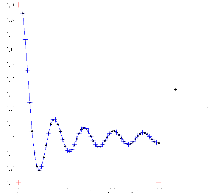
In this case, we interpolate the sinc function
def fun(x):
    return np.sin(2*np.pi*x)/(2*np.pi*x)


def grad(x):
    return np.cos(2*np.pi*x)/x - np.sin(2*np.pi*x)/(2*np.pi*x**2)
The following snippet compute the interpolation and plot it.
a = 2
b = 5
nels = 7
npts = 200
x = np.linspace(a, b, npts)
y = fun(x)
plt.plot(x, y, color="black")
xi = np.linspace(a, b, num=nels, endpoint=False)
dx = xi[1] - xi[0]
for x0 in xi:
    x1 = x0 + dx
    x = np.linspace(x0, x1, npts)
    y = hermite_interp(fun, grad, x0=x0, x1=x1, npts=npts)
plt.plot(x, y, linestyle="dashed", color="#4daf4a")
plt.plot([x[0], x[-1]], [y[0], y[-1]], marker="o", color="#4daf4a",
         linewidth=0)
plt.xlabel("x")
plt.ylabel("y")
plt.legend(["Exact function", "Interpolation"])
plt.show()