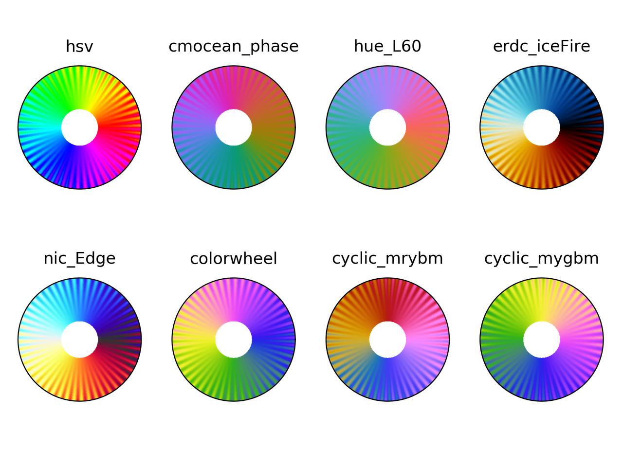
Cyclic colormaps comparison

Nicolás Guarín-Zapata

2018-01-02 18:55

Also available in:

I started this post looking for a diffusion map on Python, that I didn't find. Then I continued following an example on manifold learning by Jake Vanderplas on a different dataset. It worked nicely,

/images/manifold_learning_toroidal_helix.svg

but the colormap used is Spectral, that is divergent. This made me think about using a cyclic colormap, and ended up in this StackOverflow question. And I decided to compare some cyclic colormaps.

I picked up colormaps from different sources

cmocean:
- phase
Paraview:
- hue_L60
- erdc_iceFire
- nic_Edge
Colorcet:
- colorwheel
- cyclic_mrybm_35_75_c68
- cyclic_mygbm_30_95_c78

and, of course, hsv. You can download the colormaps in text format from here.

Comparison

For all the examples below the following imports are done:

from __future__ import division, print_function
import numpy as np
import matplotlib.pyplot as plt
from matplotlib.colors import LinearSegmentedColormap
from colorspacious import cspace_convert

Color map test image

Peter Kovesi proposed a way to compare cyclic colormaps on a paper on 2015. It consists of a spiral ramp with an undulation. In polar coordinates it reads

\begin{equation*} c = (A \rho^p \sin(n \theta) + \theta)\, \mathrm{mod}\, 2\pi \end{equation*}

with \(A\) the amplitude of the oscilation, \(\rho\) the normalized radius in [0, 1], \(p\) a positive number, and \(n\) the number of cycles.

And the following function creates the grid in Python

def circle_sine_ramp(r_max=1, r_min=0.3, amp=np.pi/5, cycles=50,
                     power=2, nr=50, ntheta=1025):
r, t = np.mgrid[r_min:r_max:nr*1j, 0:2*np.pi:ntheta*1j]
r_norm = (r - r_min)/(r_max - r_min)
vals = amp * r_norm**power * np.sin(cycles*t) + t
vals = np.mod(vals, 2*np.pi)
return t, r, vals

The following is the result

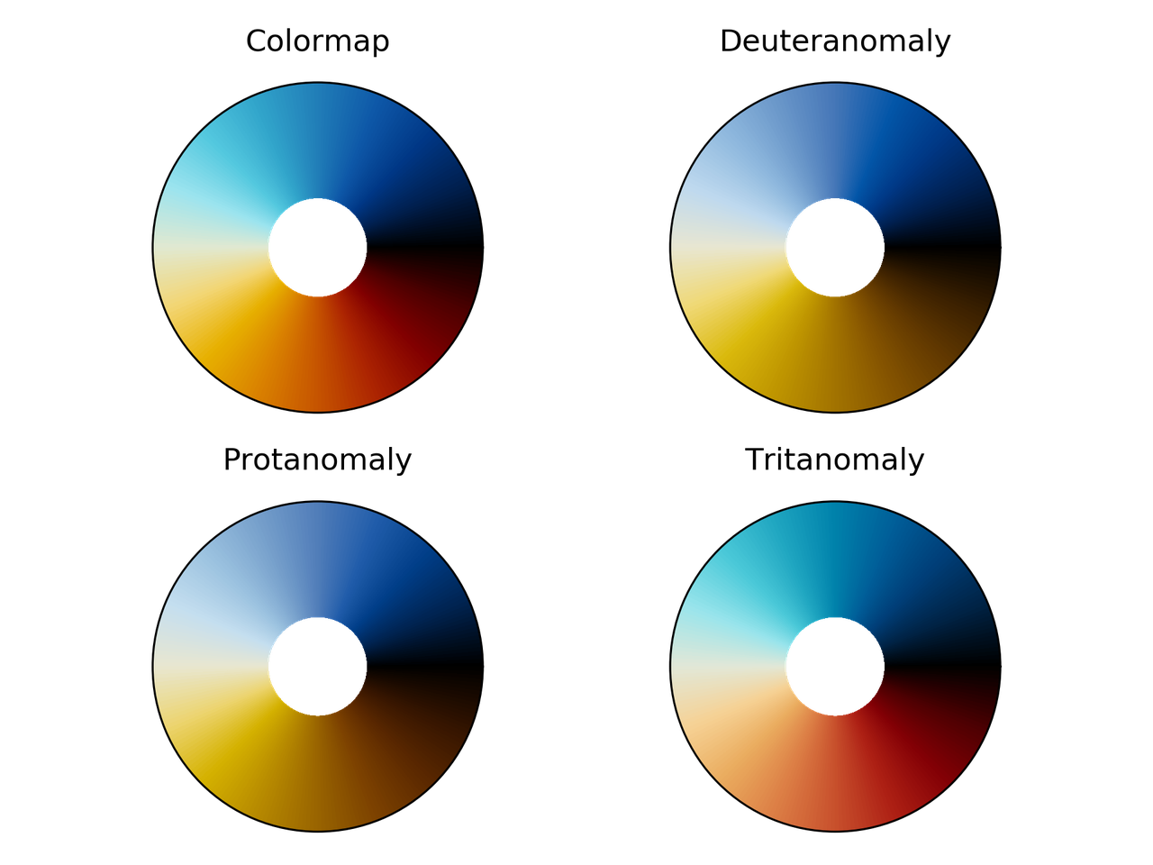
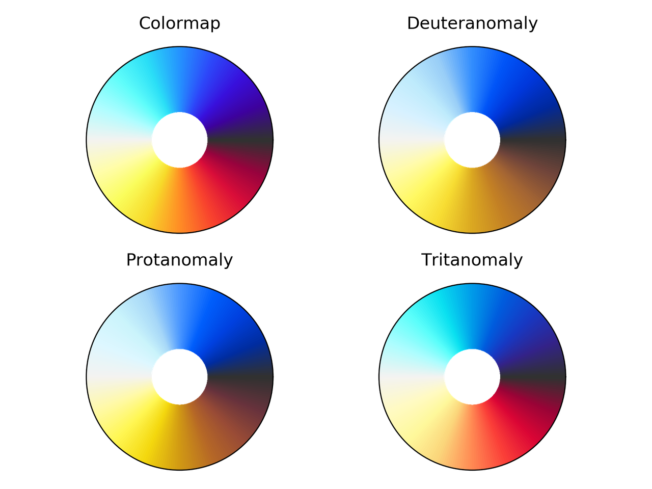
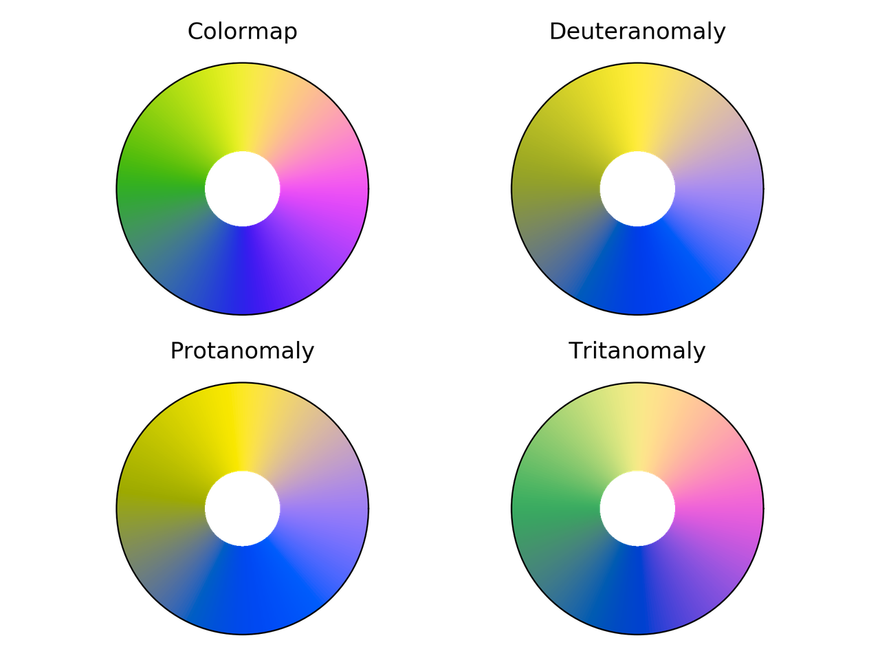
Colorblindness test

t, r, vals = circle_sine_ramp(cycles=0)
cmaps = ["hsv",
         "cmocean_phase",
         "hue_L60",
         "erdc_iceFire",
         "nic_Edge",
         "colorwheel",
         "cyclic_mrybm",
         "cyclic_mygbm"]
severity = [0, 50, 50, 50]
for colormap in cmaps:
    data = np.loadtxt(colormap + ".txt")
    fig = plt.figure()
    for cont in range(4):
        cvd_space = {"name": "sRGB1+CVD",
             "cvd_type": cvd_type[cont],
             "severity": severity[cont]}
        data2 = cspace_convert(data, cvd_space, "sRGB1")
        data2 = np.clip(data2, 0, 1)
        cmap = LinearSegmentedColormap.from_list('my_colormap', data2)
        ax = plt.subplot(2, 2, 1 + cont, projection="polar")
        ax.pcolormesh(t, r, vals, cmap=cmap)
        ax.set_xticks([])
        ax.set_yticks([])
    plt.suptitle(colormap)
    plt.tight_layout()
    plt.savefig(colormap + ".png", dpi=300)

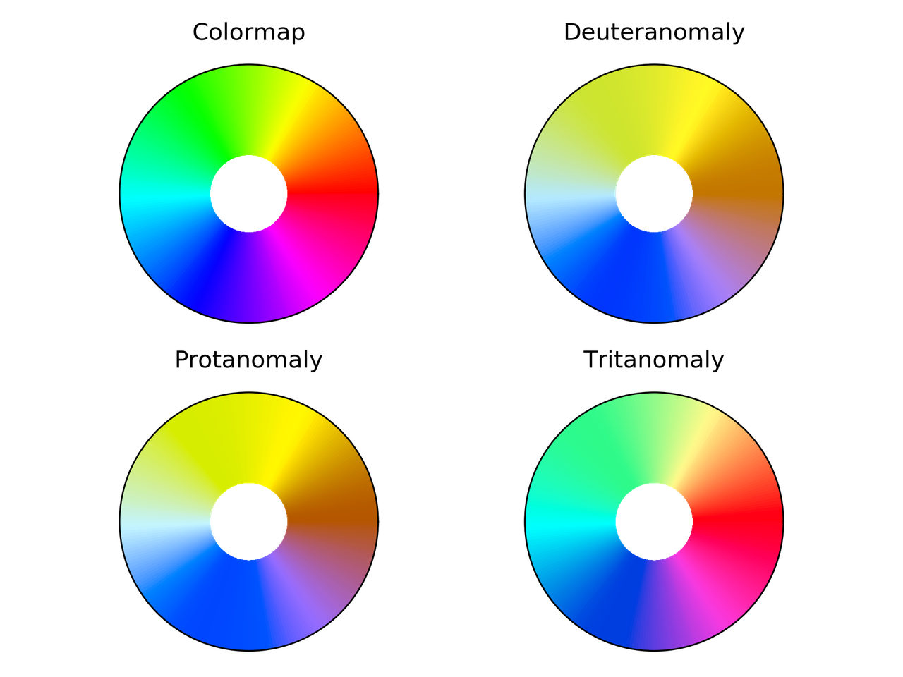
/images/hsv_eval.png — `hsv` colormap comparison for different color vision deficiencies.

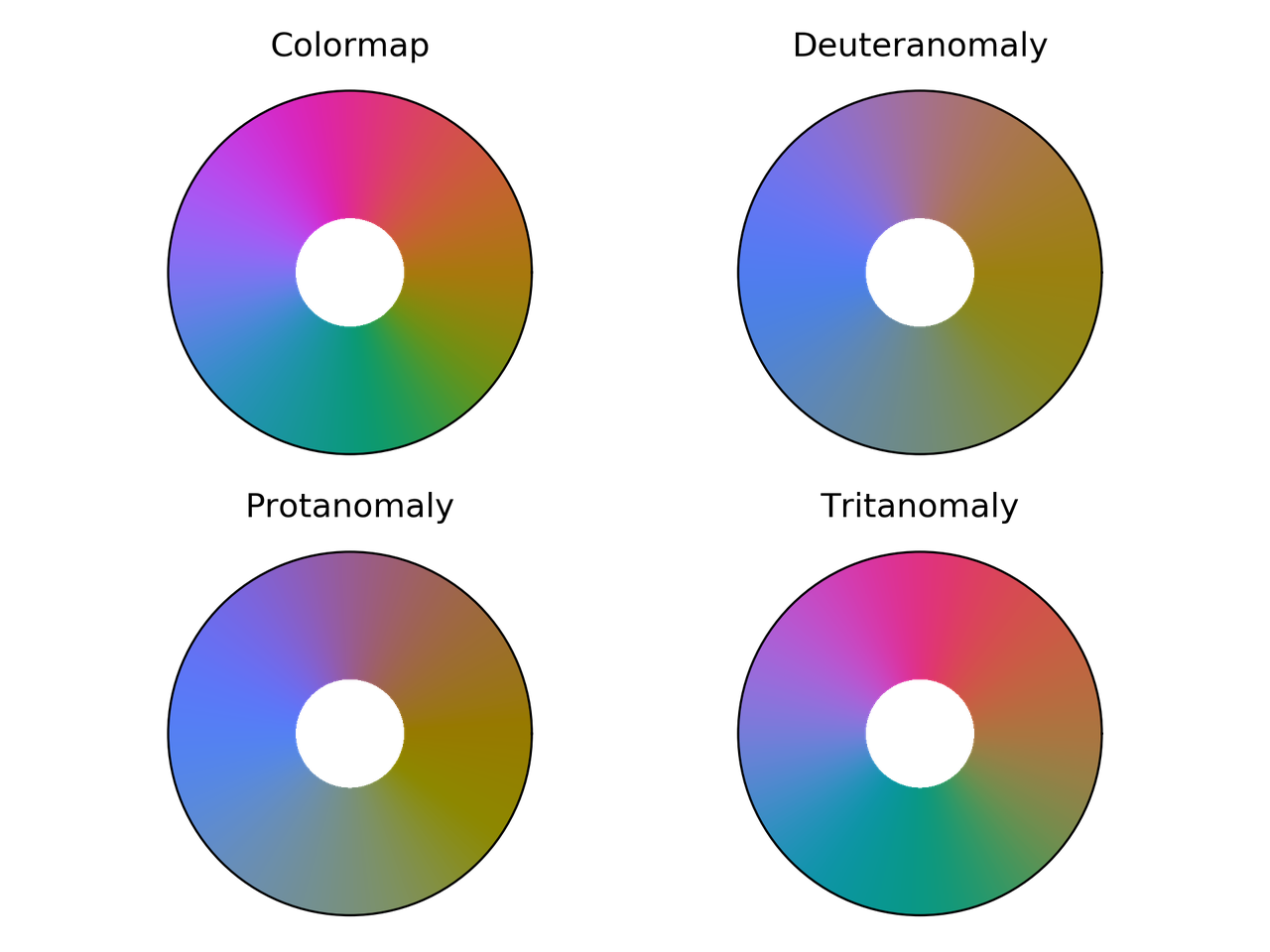
/images/cmocean_phase_eval.png — `Phase` colormap comparison for different color vision deficiencies.

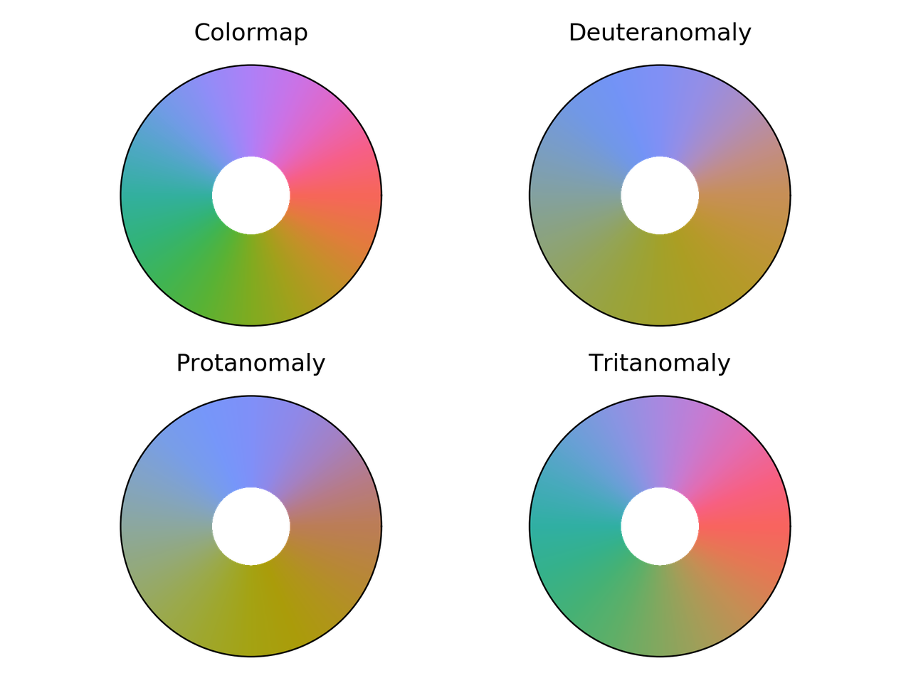
/images/hue_L60_eval.png — `hue_L60` colormap comparison for different color vision deficiencies.

/images/erdc_iceFire_eval.png — `erdc_iceFire` colormap comparison for different color vision deficiencies.

/images/nic_Edge_eval.png — `nic_Edge` colormap comparison for different color vision deficiencies.

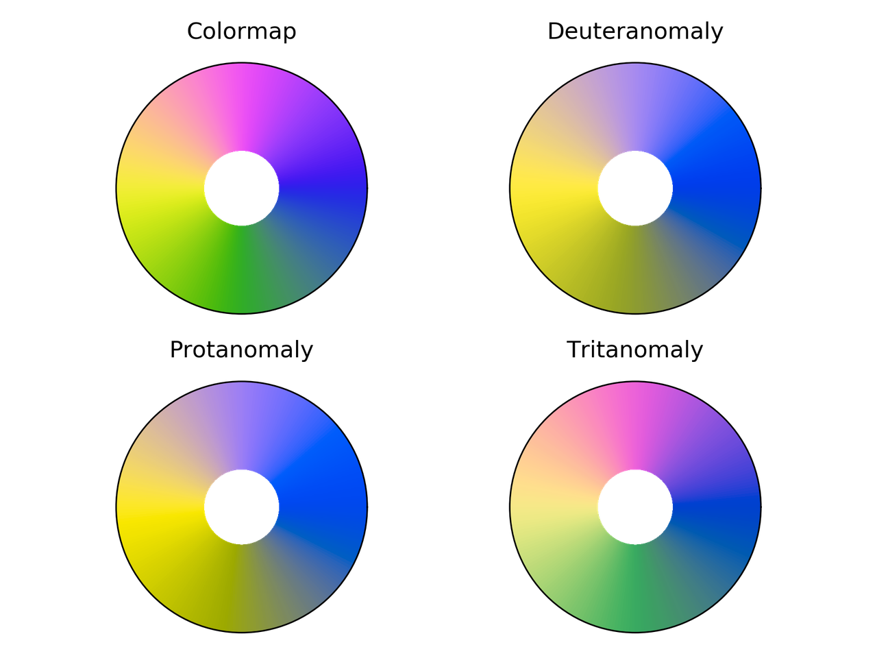
/images/colorwheel_eval.png — `Colorwheel` colormap comparison for different color vision deficiencies.

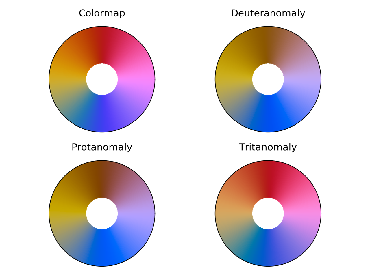
/images/cyclic_mrybm_eval.png — `Cyclic_mrybm` colormap comparison for different color vision deficiencies.

/images/cyclic_mygbm_eval.png — `Cyclic_mygbm` colormap comparison for different color vision deficiencies.

Randomly generated cyclic colormaps

What if we generate some random colormaps that are cyclic? How would they look like?

Following are the snippet and resulting colormaps.

from __future__ import division, print_function
import numpy as np
from mpl_toolkits.mplot3d import Axes3D
import matplotlib.pyplot as plt
from matplotlib.colors import LinearSegmentedColormap


# Next line to silence pyflakes. This import is needed.
Axes3D

plt.close("all")
fig = plt.figure()
fig2 = plt.figure()
nx = 4
ny = 4
azimuths = np.arange(0, 361, 1)
zeniths = np.arange(30, 70, 1)
values = azimuths * np.ones((30, 361))
for cont in range(nx * ny):
    np.random.seed(seed=cont)
    rad = np.random.uniform(0.1, 0.5)
    center = np.random.uniform(rad, 1 - rad, size=(3, 1))
    mat = np.random.rand(3, 3)
    rot_mat, _ = np.linalg.qr(mat)
    t = np.linspace(0, 2*np.pi, 256)
    x = rad*np.cos(t)
    y = rad*np.sin(t)
    z = 0.0*np.cos(t)
    X = np.vstack((x, y, z))
    X = rot_mat.dot(X) + center

    ax = fig.add_subplot(ny, nx, 1 + cont, projection='polar')
    cmap = LinearSegmentedColormap.from_list('my_colormap', X.T)
    ax.pcolormesh(azimuths*np.pi/180.0, zeniths, values, cmap=cmap)
    ax.set_xticks([])
    ax.set_yticks([])

    ax2 = fig2.add_subplot(ny, nx, 1 + cont, projection='3d')
    ax2.plot(X[0, :], X[1, :], X[2, :])
    ax2.set_xlim(0, 1)
    ax2.set_ylim(0, 1)
    ax2.set_zlim(0, 1)
    ax2.view_init(30, -60)
    ax2.set_xticks([0, 0.5, 1.0])
    ax2.set_yticks([0, 0.5, 1.0])
    ax2.set_zticks([0, 0.5, 1.0])
    ax2.set_xticklabels([])
    ax2.set_yticklabels([])
    ax2.set_zticklabels([])


fig.savefig("random_cmaps.png", dpi=300, transparent=True)
fig2.savefig("random_cmaps_traj.svg", transparent=True)

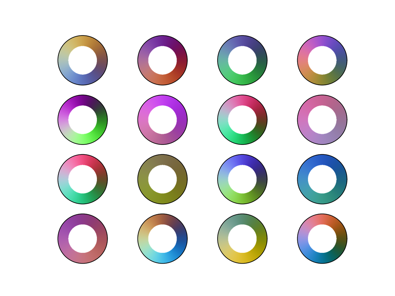
/images/random_cmaps.png — 16 randomly generated colormaps.

/images/random_cmaps_traj.svg — Trajectories in RGB space for the randomly generated colormaps.

A good idea would be to take these colormaps and optimize some perceptual parameters such as lightness to get some usable ones.

Conclusions

I probably would use phase, colorwheel, or mrybm in the future.

/images/toroidal_helix_phase.svg — Initial image using `phase`.

/images/toroidal_helix_colorwheel.svg — Initial image using `colorwheel`.

/images/toroidal_helix_mrybm.svg — Initial image using `mrybm`.

References

Peter Kovesi. Good Colour Maps: How to Design Them. arXiv:1509.03700 [cs.GR] 2015

Nicolás' blog